The Future of Doing My Programming…

As you’ve likely noticed; the pace of posts has dropped precipitously over the last few years. I’ve been completing my degree undergraduate degree in Computer Science and I had assumed that I’d have lots of things to write about in the process. Unfortunately, it turns out that most professors don’t like it when you post how to do their assignments on the Internet.

I am going to be finishing my degree in a few weeks, and after that I have a job lined up doing graphics work for a local company. I can’t imagine that my future employer will be any more excited about the prospect of me posting how they do things. Additionally, time has become a more scarce resource, and I just don’t have time for this any more.

Thus, I’m sad to say that I’ll be letting my domain subscription lapse in a few weeks. The blog will stay live at doingmyprogramming.wordpress.com, and it’s certainly possible that new posts happen. However, this is no longer something I can commit to with any sort of regularity, and I think it’s time to let go.

If you were a regular reader of mine, I wanted to say thank you. I was never doing this for money or glory, I just wanted to give something back. I know countless times I’ve had problems, and it was some blog that Google turned up that had the answer. Hopefully this blog was that result for one of you.

Reboot Early, and Often!

A wise man once said to me “Reboot early, and often!” He said it many times actually. When you’re trying to troubleshoot programs for which you don’t have the source code, you tend to develop little rituals that you go through to “fix” them…

So here I was today, trying to power through the boilerplate to draw a triangle in Vulkan. I had just finished up creating my Pipeline object, and ran my program to see if it worked. As you can imagine, it didn’t work.

Shockingly, C++ Causes Problems

First up: my shaders are invalid. The error:

validation layer: ObjectTracker : Invalid Shader Module Object 0xa.

Of course, the Object Tracker layer is there to tell you when you try to use objects that are not valid handles. Usually this is because vKcreateFoo did not return VK_SUCCESS. Of course, vkCreateShaderModule definitely did return VK_SUCCESS, because if it hadn’t my program would have died in a fire thanks to my expect assertion macro. Surely either I have a driver bug or C++ is doing “exactly what I told it to.”

So I do some troubleshooting. I upgrade my driver which does nothing. Then I examine my code. Buried in a comment thread on this stackoverflow question is the suggestion that a destructor is being called. I examine my code, and sure enough, the RAII object that I’m storing my shader in is being destructed before the call to vkCreateGraphicsPipeline. C++ was doing “exactly what I told it to.”

Sound Advice

So an hour later, and one problem down. I recompile and try again:

vkEnumeratePhysicalDevices: returned VK_ERROR_INITIALIZATION_FAILED, indicating that initialization of an object has failed

Shenanigans! There’s no way that vkEnumeratePhysicalDevices is messed up, that’s been working for weeks! I turn to the Googler, but to no avail. Then the words rang in my head “Reboot early and often!” It’s not like I just updated my graphics driver without rebooting or anything… Oh wait!

Moral of the story: reboot early, and often!

The Specter of Undefined Behavior

If you’ve ever spoken to a programmer, and really got them on a roll, they may have said the words “undefined behavior” to you. Since you speak English, you probably know what each of those words mean, and can imagine a reasonable meaning for them in that order. But then your programmer friends goes on about “null-pointer dereferencing” and “invariant violations” and you start thinking about cats or football or whatever because you are not a programmer.

I often find myself being asked what it is that I do. Since I’ve spent the last few years working on my Computer Science degree, and have spent much of that time involved in programming language research, I often find myself trying to explain this concept. Unfortunately, when put on the spot, I usually am only able to come up with the usual sort of explanation that programmers use among themselves: “If you invoke undefined behavior, anything can happen! Try to dereference a null pointer? Bam! Lions could emerge from your monitor and eat your family!” Strictly speaking, while I’m sure some compiler writer would implement this behavior if they could, it’s not a good explanation for a person who doesn’t already kind of understand the issues at play.

Today, I’d like to give an explanation of undefined behavior for a lay person. Using examples, I’ll give an intuitive understanding of what it is, and also why we tolerate it. Then I’ll talk about how we go about mitigating it.

Division By Zero

Here is one that most of us know. Tell me, what is 8 / 0? The answer of course is “division by zero is undefined.” In mathematics, there are two sorts of functions: total and partial. A total function is defined for all inputs. If you say a + b, this can be evaluated to some result no matter what you substitute for a and b. Addition is total. The same cannot be said for division. If you say a / b, this can be evaluated to some result no matter what you substitute for a and b unless you substitute b with 0. Division is not total.

If you go to the Wikipedia article for division by zero you’ll find some rationale for why division by zero is undefined. The short version is that if it were defined, then it could be mathematically proven that one equals two. This would of course imply that cats and dogs live in peace together and that pigs fly, and we can’t have that!

However, there is a way we can define division to be total that doesn’t have this issue. Instead of defining division to return a number, we could define division to return a set of numbers. You can think of a set as a collection of things. We write this as a list in curly braces. {this, is, a, set, of, words} I have two cats named Gatito and Moogle. I can have a set of cats by writing {Gatito, Moogle}. Sets can be empty; we call the empty set the null set and can write it as {} or using this symbol ∅. I’ll stick with empty braces because one of the things I hate about mathematics is everybody’s insistence on writing in Greek.

So here is our new total division function:

totalDivide(a, b)
   if (b does not equal 0)
      output {a / b}
   otherwise
      output {}

If you use totalDivide to do your division, then you will never have to worry about the undefined behavior of division! So why didn’t Aristotle (or Archimedes or Yoda or whoever invented division) define division like this in the first place? Because it’s super annoying to deal with these sets. None of the other arithmetic functions are defined to take sets, so we’d have to constantly test that the division result did not produce the empty set, and extract the result from the set. In other words: while our division is now total, we still need to treat division by zero as a special case. Let us try to evaluate 2/2 + 2/2 and totalDivide(2,2) + totalDivide(2,2):

1: 2/2 + 2/2
2: 1 + 1
3: 2

Even showing all my work, that took only 3 lines.

1: let {1} = totalDivide(2,2)
2: let {1} = totalDivide(2,2)
3: 1 + 1
4: 2

Since you can’t add two sets, I had to evaluate totalDivide out of line, and extract the values and add them separately. Even this required my human ability to look at the denominator and see that it wasn’t zero for both cases. In other words, making division total made it much more complicated to work with, and it didn’t actually buy us anything. It’s slower. It’s easier to mess up. It has no real value. As humans, it’s fairly easy for us to look at the denominator, see that it’s zero, and just say “undefined.”

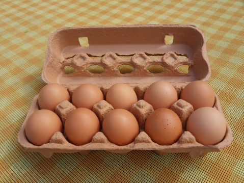
Cartons of Eggs

I’m sure many of you have a carton of eggs in your fridge. Go get me the 17th egg from your carton of eggs. Some of you will be able to do this, and some of you will not. Maybe you only have a 12 egg carton. Maybe you only have 4 eggs in your 18 egg carton, and the 17th egg is one of the ones that are missing. Maybe you’re vegan.

A basic sort of construct in programming is called an “array.” Basically, this is a collection of the same sort of things packed together in a region of memory on your computer. You can think of a carton of eggs as an array of eggs. The carton only contains one sort of thing: an egg. The eggs are all packed together right next to each other with nothing in between. There is some finite amount of eggs.

If I told you “for each egg in the carton, take it out and crack it, and dump it in a bowl starting with the first egg”, you would be able to do this. If I told you “take the 7th egg and throw it at your neighbor’s house” you would be able to do this. In the first example, you would notice when you cracked the last egg. In the second example you would make sure that there was a 7th egg, and if there wasn’t you probably picked some other egg because your neighbor is probably a jerk who deserves to have his house egged. You did this unconsciously because you are a human who can react to dynamic situations. The computer can’t do this.

If you have some array that looks like this (array locations are separated by | bars | and * stars * are outside the array) ***|1|2|3|*** and you told the computer “for each location in the array, add 1 to the number, starting at the first location” it would set the first location to be 2, the second location to be 3, the third location to be 4. Then it would interpret the bits in the location of memory directly to the right of the third location as a number, and it would add 1 to this “number” thereby destroying the data in that location. It would do this forever because this is what you told the machine to do. Suppose that part of memory was involved in controlling the brakes in your 2010 era Toyota vehicle. This is obviously incredibly bad, so how do we prevent this?

The answer is that the programmer (hopefully) knows how big the array is and actually says “starting at location one, for the next 3 locations, add one to the number in the location”. But suppose the programmer messes up, and accidentally says “for the next 4 locations” and costs a multinational company billions of dollars? We could prevent this. There are programming languages that give us ways to prevent these situations. “High level” programming languages such as Java have built-in ways to tell how long an array is. They are also designed to prevent the programmer from telling the machine to write past the end of the array. In Java, the program will successfully write |2|3|4| and then it will crash, rather than corrupting the data outside of the array. This crash will be noticed in testing, and Toyota will save face. We also have “low level” programming languages such as C, which don’t do this. Why do we use low level programming languages? Let’s step through what these languages actually have the machine do for “starting at location one, for the next 3 locations, add one to the number in the location”: First the C program:

NOTE: location[some value] is shorthand for “the location identified by some value.” egg_carton[3] is the third egg in the carton. Additionally, you should read these as sequential instructions “first do this, then do that” Finally, these examples are greatly simplified for the purposes of this article.

1: counter = 1
2: location[counter] = 1 + 1
3: if (counter equals 3) terminate
4: counter = 2
5: location[counter] = 2 + 1
6: if (counter equals 3) terminate
7: counter = 3
8: location[count] = 3 + 1
9: if (counter equals 3) terminate

Very roughly speaking, this is what the computer does. The programmer will use a counter to keep track of their location in the array. After updating each location, they will test the counter to see if they should stop. If they keep going they will repeat this process until the stop condition is satisfied. The Java programmer would write mostly the same program, but the program that translates the Java code into machine code (called a compiler) will add some stuff:

1: counter = 1
2: if (counter greater than array length) crash
3: location[counter] = 1 + 1
4: if (counter equals 3) terminate
5: counter = 2
6: if (counter greater than array length) crash
7: location[counter] = 2 + 1
8: if (counter equals 3) terminate
9: counter = 3
10: if (counter greater than array length) crash
11: location[count] = 3 + 1
12: if (counter equals 3) terminate

As you can see, 3 extra lines were added. If you know for a fact that the array you are working with has a length that is greater than or equal to three, then this code is redundant.

For such a small array, this might not be a huge deal, but suppose the array was a billion elements. Suddenly an extra billion instructions were added. Your phone’s processor likely runs at 1-3 gigahertz, which means that it has an internal clock that ticks 1-3 billion times per second. The smallest amount of time that an instruction can take is one clock cycle, which means that in the best case scenario, the java program takes one entire second longer to complete. The fact of the matter is that “if (counter greater than array length) crash” definitely takes longer than one clock cycle to complete. For a game on your phone, this extra second may be acceptable. For the onboard computer in your car, it is definitely not. Imagine if your brakes took an extra second to engage after you push the pedal? Congressmen would get involved!

In Java, reading off the end of an array is defined. The language defines that if you attempt to do this, the program will crash (it actually does something similar but not the same, but this is outside the scope of this article). In order to enforce this definition, it inserts these extra instructions into the program that implement the functionality. In C, reading off the end of an array is undefined. Since C doesn’t care what happens when you read off the end of an array, it doesn’t add any code to your program. C assume you know what you’re doing, and have taken the necessary steps to ensure your program is correct. The result is that the C program is much faster than the Java program.

There are many such undefined behaviors in programming. For instance, your computer’s division function is partial just like the mathematical version. Java will test that the denominator isn’t zero, and crash if it is. C happily tells the machine to evaluate 8 / 0. Most processors will actually go into a failure state if you attempt to divide by zero, and most operating systems (such as Windows or Mac OSX) will crash your program to recover from the fault. However, there is no law that says this must happen. I could very well create a processor that sends lions to your house to punish you for trying to divide by zero. I could define x / 0 = 17. The C language committee would be perfectly fine with either solution; they just don’t care. This is why people often call languages such as C “unsafe.” This doesn’t mean that they are bad necessarily, just that their use requires caution. A chainsaw is unsafe, but it is a very powerful tool when used correctly. When used incorrectly, it will slice your face off.

What To Do

So, if defining every behavior is slow, but leaving it undefined is dangerous, what should we do? Well, the fact of the matter is that in most cases, the added overhead of adding these extra instructions is acceptable. In these cases, “safe” languages such as Java are preferred because they ensure program correctness. Some people will still write these sorts of programs in unsafe languages such as C (for instance, my own DMP Photobooth is implemented in C), but strictly speaking there are better options. This is part of the explanation for the phenomenon that “computers get faster every year, but [insert program] is just as slow as ever!” Since the performance of [insert program] we deemed to be “good enough”, this extra processing power is instead being devoted to program correctness. If you’ve ever used older versions of Windows, then you know that your programs not constantly crashing is a Good Thing.

This is fine and good for those programs, but what about the ones that cannot afford this luxury? These other programs fall into a few general categories, two of which we’ll call “real-time” and “big data.” These are buzzwords that you’ve likely heard before, “big data” programs are the programs that actually process one billion element arrays. An example of this sort of software would be software that is run by a financial company. Financial companies have billions of transactions per day, and these transactions need to post as quickly as possible. (suppose you deposit a check, you want those funds to be available as quickly as possible) These companies need all the speed they can get, and all those extra instructions dedicated to totality are holding up the show.

Meanwhile “real-time” applications have operations that absolutely must complete in a set amount of time. Suppose I’m flying a jet, and I push the button to raise a wing flap. That button triggers an operation in the program running on the flight computer, and if that operation doesn’t complete immediately (where “immediately” is some fixed, non-zero-but-really-small amount of time) then that program is not correct. In these cases, the programmer needs to have very precise control over what instructions are produced, and they need to make every instruction count. In these cases, redundant totality checks are a luxury that is not in the budget.

Real-time and big data programs need to be fast, so they are often implemented in unsafe languages, but that does not mean that invoking undefined behavior is OK. If a financial company sets your account balance to be check value / 0, you are not going to have a good day. If your car reads the braking strength from a location off to the right of the braking strength array, you are going to die. So, what do these sorts of programs do?

One very common method, often used in safety-critical software such as a car’s onboard computer is to employ strict coding standards. MISRA C is a set of guidelines for programming in C to help ensure program correctness. Such guidelines instruct the developer on how to program to avoid unsafe behavior. Enforcement of the guidelines is ensured by peer-review, software testing, and Static program analysis.

Static program analysis (or just static analysis) is the process of running a program on a codebase to check it for defects. For MISRA C, there exists tooling to ensure compliance with its guidelines. Static analysis can also be more general. Over the last year or so, I’ve been assisting with a research project at UCSD called Liquid Haskell. Simply put, Liquid Haskell provides the programmer with ways to specify requirements about the inputs and outputs of a piece of code. Liquid Haskell could ensure the correct usage of division by specifying a “precondition” that “the denominator must not equal zero.” (I believe that this actually comes for free if you use Liquid Haskell as part of its basic built-in checks) After specifying the precondition, the tool will check your codebase, find all uses of division, and ensure that you ensured that zero will never be used as the denominator.

It does this by determining where the denominator value came from. If the denominator is some literal (i.e. the number 7, and not some variable a that can take on multiple values), it will examine the literal and ensure it meets the precondition of division. If the number is an input to the current routine, it will ensure the routine has a precondition on that value that it not be zero. If the number is the output from some other routine, it verifies that the the routine that produced the value has, as a “postcondition”, that its result will never be zero. If the check passes for all usages of division, your use of division will be declared safe. If the check fails, it will tell you what usages were unsafe, and you will be able to fix it before your program goes live. The Haskell programming language is very safe to begin with, but a Haskell program verified by Liquid Haskell is practically Fort Knox!

The Human Factor

Humans are imperfect, we make mistakes. However, we make up for it in our ability to respond to dynamic situations. A human would never fail to grab the 259th egg from a 12 egg carton and crack it into a bowl; the human wouldn’t even try. The human can see that there is only 12 eggs without having to be told to do so, and will respond accordingly. Machines do not make mistakes, they do exactly what you tell them to, exactly how you told them to do it. If you tell the machine to grab the 259th egg and crack it into a bowl, it will reach it’s hand down, grab whatever is in the space 258 egg lengths to the right of the first egg, and smash it on the edge of a mixing bowl. You can only hope that nothing valuable was in that spot.

Most people don’t necessarily have a strong intuition for what “undefined behavior” is, but mathematicians and programmers everywhere fight this battle every day.

Onwards To The Moon

As the deadline looms, work continues at a feverish pace. Much has happened, and much remains to be done.

Procedural Terrain Generation

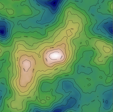
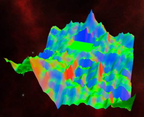
The terrain generation is basically done. We are generating random landscape heightmaps using the Diamond-Square algorithm. After generating the heightmaps, we carve out a flat space for the city, and then place various mineral deposits and crystal growths. After the features are set, we tessellate the landscape.

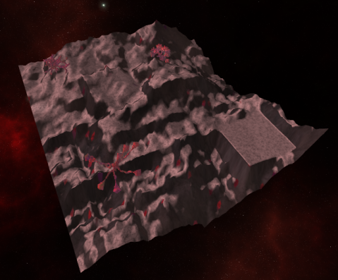
We are also capable of reading in external heightmap data, and I’ve located a heightmap of the surface of the moon, which we are capable of turning into a 3D surface.

As you can see, the lunar surface is much rougher than one would think.

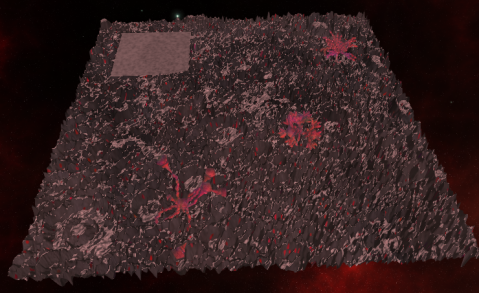
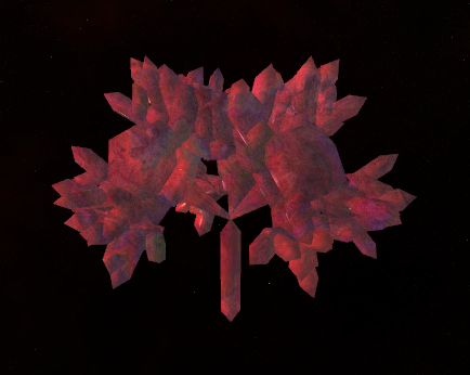
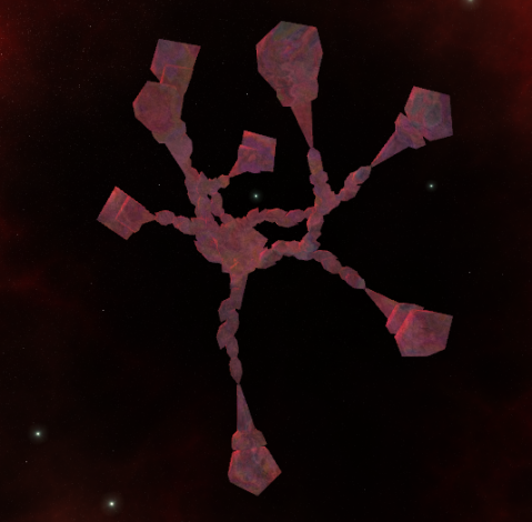
Crystalline Structures

New this week are the crystalline structures seen in the screenshots above. These are generated using L-systems, with the following grammar:

V = { D(len, topScale, bottomScale, topLen, bottomLen),
      C(len, topScale, bottomScale, topLen, bottomLen),
      S(scale),
      T(minSegs) }
S = { F(theta),
      K(theta),
      A(r, s) }
ω1 = { A(C(6,1,1,1,1), D(1.0f, 3.0f, 2.5f, 0.5f, 1.0f)) }
ω2 = { A(C(6,1,1,1,1), A(F(1), S(1))) }
ω3 = { A(S(1), A(K(1), T(3)) }
P = { D -> A(D, A((K(1), C(2,1,1,1,1)))),
      C -> A(C, A(F(0.75), T(3))),
      T : final iteration -> A(T, S(0.5)),
      T : otherwise       -> A(T, T(1)),
      S : -> A(S, D(3,2,1,1,1)) }

There is a basic crystal building block, represented by D and C. These are the same shape, but D has 5 branching points, and C has 1 (the center.) To build on a mounting point, one uses the A rule, which states “For all mounting points produced by r, build s on it.”

Rounding out the bunch, are S a “scepter” shaped crystal, F, which fans out in three directions, and K, which forks in two directions. Last but not least is the “angry tentacle” formation T.

Here we see ω1:

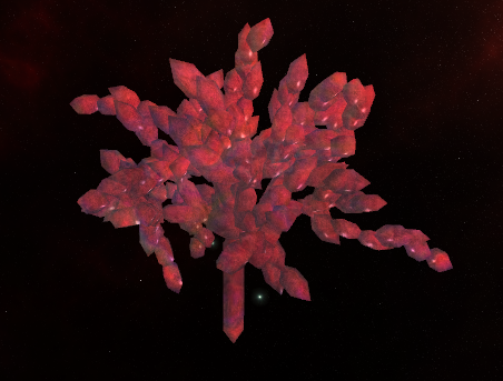
… ω2:

…and ω3:

Procedural City Generation

We’ll be placing a procedurally generated moon base on the flat build site carved out of the terrain. The moon’s surface is very rough, so we can only place the base on the flat area.

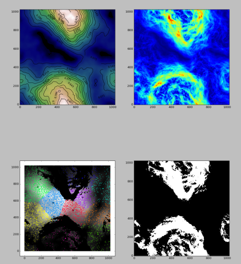
However, the area under the city isn’t completely flat; we are using a technique called spectral synthesis to generate a smoother heightmap underneath the city. The edges of this heightmap will coincide smoothly with the surrounding terrain to ensure a natural transition.

After generating the heightmaps, we generate a population density map using a similar procedure, attenuating it where the terrain is steepest (it’s difficult to build on the side of a hill!). Then we sample the density map and place population centers using k-means clustering. Finally, we triangulate the set of population centers to generate a connectivity graph for road generation.

Once we have a connectivity graph, we draw adaptive highways between population centers using the technique described in Citygen: An Interactive System for Procedural City Generation, using a heuristic combining Least Elevation Difference, population density, and the degree to which the road would deviate from its current direction. As these are drawn, we create additional perpendicular roads in areas of high population density. These roads are extended using the same heuristic until they reach a less populated area.

So far, we’ve implemented the above in Python so we can leverage the performant array operations from NumPy and SciPy, in addition to the spatial indexing functionality from Rtree. We’ll need to use the Python C API to call into our Python code and store the resulting road graph in a buffer for rendering.

The Way Ahead

Much work remains to be done. For terrain and L-systems, there remains polish work. I’ve implemented the required algorithms, and it technically “works.” However, it’s still a bit rough. I hope to refine the shaders of the crystals to make them appear more 3-dimensional. Additionally, I’d like to increase the density of “trees” on the landscape as I think it looks a bit sparse. I hope to have this work wrapped up by tomorrow night.

For city generation, the road graph needs to be converted to buildable cells, and subdivided/populated with buildings. Andrew plans to have this done by tomorrow night. By Sunday, he plans to have the rendering set up for this, with basic buildings. Then by Monday, more elaborate buildings will follow.

Additionally, we need the capability to regenerate the various procedurally generated components at runtime. This is a simple matter of plumbing, and should not be difficult. Time allowing, I’d like to do this asynchronously, so there is no frame hiccup during regeneration. The user will press a button, and a few seconds later, the change will be reflected.

Procedural Moonbase

Having reached the end of UCSD’s Intro to Computer Graphics course, I have been tasked with creating a real-time demo that implements a subset of features covered in the class. Today is the first of three posts about the progress of this project.

For this project myself (Chris Tetreault) and my partner Andrew Buss will be implementing 4 features:

• Procedurally modelled city
• Procedurally modelled buildings
• Procedurally generated terrain
• Procedurally generated “plants” with L-systems

With all of these, we’ll be creating a procedurally generated moon base. First, we will generate a landscape, and carve out a flat spot for the base. Next, we will generate a city, which consists of a procedurally generated layout populated by procedurally generated buildings. Finally, we will procedurally generate doodads to be placed on the landscape throughout the undeveloped portion of the terrain.

All of this will be implemented in modern C++ with modern OpenGL.

Terrain and “Plants”

This portion of the project is coming along nicely. We are currently generating the landscape, with the exception of textures. We currently have the surface normals set as the pixel color in the fragment shader.

At some elevation lower than the city, I plan to add lava. Additionally, I plan to have two land based-textures that I will select between based on the elevation gain. Likely, this will be a smooth rock texture for steep hills, and gravel for flatter areas.

After completing this, I will use L-systems to generate stuff to put on the landscape. This will likely take the form of geological formations, such as rocks or lava flows as one isn’t likely to find trees on a blasted lunar wasteland.

Cities and Buildings

For the city portion, we’ll be procedurally generating moon base buildings. We decided to go with the moon base, as opposed to a traditional city because we felt this could give us more creative freedom to do what we want. After all; if the task is to procedurally generate a “City”, how many urban downtown areas are you likely to see?

This portion of the project is still in the planning phase, so expect to see more on this next week.

Aeson Revisited

As many of you know, the documentation situation in Haskell leaves something to be desired. Sure, if you are enlightened, and can read the types, you’re supposedly good. Personally, I prefer a little more documentation than “clearly this type is a monoid in the category of endofunctors”, but them’s the breaks.

Long ago, I wrote about some tricks I found out about using Aeson, and I found myself using Aeson again today, and I’d like to revisit one of my suggestions.

Types With Multiple Constructors

Last time we were here, I wrote about parsing JSON objects into Haskell types with multiple constructors. I proposed a solution that works fine for plain enumerations, but not types with fields.

Today I had parse some JSON into the following type:

data Term b a =
   App b [Term b a]
   | Var VarId
   | UVar a

I thought “I’ve done something like this before!” and pulled up my notes. They weren’t terribly helpful. So I delved into the haddocs for Aeson, and noticed that Aeson's Result type is an instance of MonadPlus. Could I use mplus to try all three different constructors, and take whichever one works?

instance (FromJSON b, FromJSON a)
         => FromJSON (Term b a) where
   parseJSON (Object v) = parseVar `mplus` parseUVar
                                   `mplus` parseApp
      where
         parseApp = do
            ident <- v .: "id"
            terms <- v .: "terms"
            return $ App ident terms
         parseVar = Var <$> v .: "var"
         parseUVar = UVar <$> v .: "uvar"
   parseJSON _ = mzero

It turns out that I can.

Baby’s First Proof

Unlike many languages that you learn, in Coq, things are truly different. Much like your first functional language after using nothing but imperative languages, you have to re-evaluate things. Instead of just defining functions, you have to prove properties of them. So, let’s take a look at a few basic ways to do that.

Simpl and Reflexivity

Here we have two basic “tactics” that we can use to prove simple properties. Suppose we have some function addition. We’re all familiar with how this works; 2 + 2 = 4, right? Prove it:

Lemma two_plus_two:
  2 + 2 = 4.
Proof.
  Admitted.

First, what is this Admitted. thing? Admitted basically tells Coq not to worry about it, and just assume it is true. This is the equivalent of your math professor telling you “don’t worry about it, Aristotle says it’s true, are you calling Aristotle a liar?” and if you let this make it into live code, you are a bad person. We must make this right!

Lemma two_plus_two:
  2 + 2 = 4.
Proof.
  simpl.
  reflexivity.
Qed.

That’s better. This is a simple proof; we tell Coq to simplify the expression, then we tell Coq to verify that the left-hand-side is the same as the right-hand-side. One nice feature of Coq is that lets you step through these proofs to see exactly how the evaluation is proceeding. If you’re using Proof General, you can use the buttons Next, Goto, and Undo to accomplish this. If you put the point at Proof. and click Goto, Coq will evaluate the buffer up to that point, and a window should appear at the bottom with the following:

1 subgoals, subgoal 1 (ID 2)

  ============================
   2 + 2 = 4

This is telling you that Coq has 1 thing left to prove: 2 + 2 = 4. Click next, the bottom should change to:

1 subgoals, subgoal 1 (ID 2)

  ============================
   4 = 4

Coq processed the simpl tactic and now the thing it needs to prove is that 4 = 4. Obviously this is true, so if we click next…

No more subgoals.

…reflexivity should succeed, and it does. If we click next one more time:

two_plus_two is defined

This says that this Lemma has been defined, and we can now refer to it in other proofs, much like we can call a function. Now, you may be wondering “do I really have to simplify 2 + 2?” No, you don’t, reflexivity will simplify on it’s own, this typechecks just fine:

Lemma two_plus_two:
  2 + 2 = 4.
Proof.
  reflexivity.
Qed.

So, what’s the point of simpl then? Let’s consider a more complicated proof.

Induction

Lemma n_plus_zero_eq_n:
  forall (n : nat), n + 0 = n.

This lemma state that for any n, n + 0 = n. This is the same as when you’d write ∀ in some math. Other bits of new syntax is n : nat, which means that n has the type nat. The idea here is that no matter what natural number n is, n + 0 = n. So how do we prove this? One might be tempted to try:

Lemma n_plus_zero_eq_n:
  forall (n : nat), n + 0 = n.
Proof.
  reflexivity.
Qed.

One would be wrong. What is Coq stupid? Clearly n + 0 = n, Aristotle told me so! Luckily for us, this is a pretty easy proof, we just need to be explicit about it. We can use induction to prove this. Let me show the whole proof, then we’ll walk through it step by step.

Lemma n_plus_zero_eq_n:
  forall (n : nat), n + 0 = n.
Proof.
  intros n.
  induction n as [| n'].
  {
    reflexivity.
  }
  {
    simpl.
    rewrite -> IHn'.
    reflexivity.
  }
Qed.

Place the point at Proof and you’ll see the starting goal:

1 subgoals, subgoal 1 (ID 6)

  ============================
   forall n : nat, n + 0 = n

Click next and step over intros n.

1 subgoals, subgoal 1 (ID 7)

  n : nat
  ============================
   n + 0 = n

What happened here is intros n introduces the variable n, and names it n. We could have done intros theNumber and the bottom window would instead show:

1 subgoals, subgoal 1 (ID 7)

  theNumber : nat
  ============================
   theNumber + 0 = theNumber

The intros tactic reads from left to right, so if we had some Lemma foo : forall (n m : nat), [stuff], we could do intros nName mName., and it would read in n, and bind it to nName, and then read in m and bind it to mName. Click next and evaluate induction n as [| n'].

2 subgoals, subgoal 1 (ID 10)

  ============================
   0 + 0 = 0

subgoal 2 (ID 13) is:
 S n' + 0 = S n'

The induction tactic implements the standard proof by induction, splitting our goal into two goals: the base case and the n + 1 case. Similarly to intros, this will create subgoals starting with the first constructor of an ADT, and ending with the last.

On Natural Numbers in Coq

Let us take a second to talk about how numbers are represented in Coq. Coq re-implements all types within itself, so nat isn’t a machine integer, it’s an algebraic datatype of the form:

Inductive nat : Set :=
  | O : nat
  | S : nat -> nat.

O is zero, S O is one, and S (S (S (O))) is three. There is a lot of syntax sugar in place that lets you write 49 instead of S (S ( ... ( S O) ... )), and that’s a good thing.

The point of all of this is that we can pattern match on nat much like we can a list.

More Induction

…anyways, all this brings us back to induction and this mysterious as [| n']. What this is doing is binding names to all the fields of the ADT we are deconstructing. The O constructor takes no parameters, so there is nothing to the left of the |. The S constructor takes a nat, so we give it the name n'. Click next and observe the bottom change:

1 focused subgoals (unfocused: 1)
, subgoal 1 (ID 10)

  ============================
   0 + 0 = 0

The curly braces “focuses” the current subgoal, hiding all irrelevant information. Curly braces are optional, but I find them to be very helpful as the bottom window can become very cluttered in large proofs. Here we see the base case goal being to prove that 0 + 0 = 0. Obviously this is true, and we can have Coq verify this by reflexivity. Click next until the next opening curly brace is evaluated. We see the next subgoal:

1 focused subgoals (unfocused: 0)
, subgoal 1 (ID 13)

  n' : nat
  IHn' : n' + 0 = n'
  ============================
   S n' + 0 = S n'

So, what do we have here? This is the n + 1 case; here the n’ in S n' is the original n. A particularly bored reader may try to prove forall (n : nat), S n = n + 1 and I’ll leave that as an exercise. However, this follows from the definition of nat.

Also of note here is IHn'. IH stands for induction hypothesis, and this is that n’ + 0 = n’. So, how do we proceed? Click next and observe how the subgoal changes:

1 focused subgoals (unfocused: 0)
, subgoal 1 (ID 15)

  n' : nat
  IHn' : n' + 0 = n'
  ============================
   S (n' + 0) = S n'

It brought the + 0 inside the S constructor. Notice that now there is n' + 0 on the left hand side. Click next and watch closely what happens:

1 focused subgoals (unfocused: 0)
, subgoal 1 (ID 16)

  n' : nat
  IHn' : n' + 0 = n'
  ============================
   S n' = S n'

Here we use the induction hypothesis to rewrite all occurrences of n' + 0, which was the left hand side of the induction hypothesis as n', which was the right hand side of the induction hypothesis. This is what the rewrite tactic does. Notice now that the subgoal is S n' = S n' which reflexivity will surely find to be true. So, what would happen if we had done rewrite <- IHn'.?

1 focused subgoals (unfocused: 0)
, subgoal 1 (ID 16)

  n' : nat
  IHn' : n' + 0 = n'
  ============================
   S (n' + 0 + 0) = S (n' + 0)

It rewrote all instances of n', which was the right hand side of the induction hypothesis with n' + 0 which was the left hand side of the induction hypothesis. Obviously, this isn’t what we want. I should note that you can undo this by rewriting to the right twice…

  {
    simpl.
    rewrite <- IHn'.
    rewrite -> IHn'.
    rewrite -> IHn'.
    reflexivity.
  }

…and it will technically work. But don’t do this, it’s silly and there’s no room for silliness in a rigorous mathematical proof.

Personally, I have a hard time keeping it straight what the left and right rewrites do. I sometimes find myself just trying one, and then the other if I guessed wrong. Think of it like this: rewrite -> foo rewrites the current goal, replacing all occurrences of the thing on the left hand side of the equation of foo with the thing on the right hand side of the equation. It changes from the left to the right. And vice-versa for rewrite <-, which changes from the right to the left.

Random Operators: How to Make Friends and Influence Your Co-workers

If you were to ask me what language does operator overloading right, my unqualified answer would be Haskell. Unlike many languages, such as Rust or C++, operators aren’t these special things. They are just functions. Also, unlike many languages, you can define any arbitrary operator.

Now, ask me what I think is a major issue with Haskell. Do it. I dare you.

Well, if you insist…

A major issue I have with Haskell is that there are too many operators! Hundreds in base, and every library author thinks it’s ok to create hundreds more! Unfortunately, such is life; might as well get used to it.

There are two operators in particular that are quite prolific, and I think worthy of further discussion: . and $.

Function Composition

Here is the type of . :

(.) :: (b -> c) -> (a -> b) -> a -> c

. is the function composition operator. Take a function f :: a -> b and a function g :: b -> c, you can create a function fg :: a -> c:

fg :: a -> c
fg = g . f

You can chain these together too. Let h :: c -> d, i :: d -> e, and just for fun j :: e -> a:

funWithCategories :: a -> a
funWithCategories = j . i . h . g . f

Try it with your friends! They’ll love you!

I know, it was hard for me to write too, but I’ll be darned if it doesn’t look good! Just replace the . with “after”, and read it out loud:

"j after i after h after g after f"

Or, if you prefer to look at code:

funWithCategories :: a -> a
funWithCategories a = j (i (h (g (f a))))

… or in C:

a fun_with_categories(a input)
{
   return j(i(h(g(f(input)))));
}

Function Application

Now, let’s talk about $ the function application operator. Here is the type of $ :

($) :: (a -> b) -> a -> b

Basically it applied its right hand side argument to the left hand side function. Thus show 1 is the same thing as show $ 1. However, there’s a twist. Function application in Haskell is the highest precedence thing that can happen. This means that we often have to use a lot of parenthesis to make our code compile. Say I wanted to convert the output of 2 + 2. This won’t work:

Prelude> show 2 + 2

<interactive>:25:8:
    No instance for (Num String) arising from a use of ‘+’
    In the expression: show 2 + 2
    In an equation for ‘it’: it = show 2 + 2

What actuall happened was:

(show 2) + 2

…and that’s just silly. To make this code compile, we have to add parenthesis:

Prelude> show (2 + 2)
"4"

which is kind of annoying. However, we can use $ to eliminate these parenthesis!

Prelude> show $ 2 + 2
"4"

The function application operator has a precedence of 0, so the addition happens first! It has a right fixity so you can chain it!

funWithOperators :: a -> a
funWithOperators a = j $ i $ h $ g $ f a

Hey, I’ve Seen That Function Before!

If this looks familiar to you, then you’ve been paying attention!

($) ::             (a -> b) -> a -> b
(.) :: (b -> c) -> (a -> b) -> a -> c

If you chop off the first argument of . and squint, they kind of look the same. Logically, they can often be used interchangeably, however you will end up using some parenthesis with ..

My advice:

Use $ if you’re trying to produce a value for use right now. If you find yourself doing something like this:

show (show ( show( show "catcatcatcat")))

… then change it to this and save yourself the hassle of counting parenthesis:

show $ show $ show $ show "catcatcatcat"

Use . when you’re trying to make a function. If you find yourself doing something like this:

showWith :: (Show a) => (a -> String) -> a -> String
showWith = -- stuff

shower :: (Show a) => a -> String
shower a = show $ show $ show $ show a

showWith shower "catcatcatcat"

… then you can avoid defining shower like so:

showWith (show . show . show . show) "catcatcatcat"

Might It Be Case Sensitive?

So today I thought I’d mess around with the new SDL2 Bindings for Haskell.

I set up a cabal project and added my build-depends:

build-depends: base >=4.8 && <4.9, sdl2 >= 2, openglraw

OK! Let’s do this!

$ cabal install
Resolving dependencies...
cabal: Could not resolve dependencies:
trying: gl-tut-0.1.0.0 (user goal)
next goal: openglraw (dependency of gl-tut-0.1.0.0)
Dependency tree exhaustively searched.

Note: when using a sandbox, all packages are required to have consistent
dependencies. Try reinstalling/unregistering the offending packages or
recreating the sandbox.

What is this nonsense? No possible build plan? I don’t believe it!

$ cabal install sdl2-2.0.0 openglraw
Resolving dependencies...
Notice: installing into a sandbox located at

...

OK, that works…

Maybe it’s magically case sensitive?

build-depends: base >=4.8 && <4.9, sdl2 >= 2.0, OpenGLRaw

…work this time you POS! I COMMAND YOU!

$ cabal install
Resolving dependencies...
Notice: installing into a sandbox located at

...

…and of course it works…

It turns out that cabal packages can be case sensitive. Sometimes.

Do We Really Need All These Monad Transformers?

Since I first learned about them, I’ve been a fan of Monad Transformers. Just stick them all together and we can pretend we’re writing Java, who doesn’t want that? Mutable State, Logging, Configuration, Exceptions, they’re all there. Heck, stick some IO in that if you like. Apparently, there’s even a pre-built Reader/Writer/State Monad in there. However, lately I’ve been working on a fairly large Haskell project, and this project doesn’t use Monad transformers. And you know what? It’s working out for them just fine.

Lately, I’ve been wondering if all these transformers are really worth the effort? After you’ve chained together some massive runFoo (runBar (runBaz (runMonadRun ))) foobarbaz function, and got it all working right and not returning some ridiculous nested tuple, what have you gained?

ReaderT

First up is ReaderT. ReaderT let’s us carry around a read-only configuration. In an ReaderT Monad, we can do the following:

foo :: (MonadReader c m) => a -> m b
foo a = do -- stuff
           config <- ask
           -- more stuff, presumably using config

…without having to have a config parameter on our function. This is nice because it improves readability. Right? Because this is so bad:

foo :: c -> a -> b
foo c a = -- stuff, presumably using config

“But ReaderT gets you local!” you say:

foo :: (MonadReader c m) => a -> m b
foo a = do -- stuff
           local modifyC bar
   where
      modifyC c = -- change the config
      bar = -- some monad

Nifty, I agree. Or we chould just do:

foo :: c -> a -> b
foo c a = bar (modifyC c)
   where
      modifyC c = -- change the config
      bar c = -- some function of c

…which I believe is much clearer, because I didn’t have to go to Hackage to figure out what local does.

StateT

Conceptually kind of a combination of ReaderT and WriterT (I’m going to skip WriterT for the sake of brevity), StateT lets us use mutable state in a Monadic function:

foo :: (MonadState s m) => a -> m b
foo a = do state <- get
        -- do stuff, presumably change the state
        put state'
        -- more stuff

So, what’s the non-monadic alternative? I imagine something like this:

foo :: s -> a -> (s, b)
foo s a = (s', a')
   where
      s' = -- do something to change the state
      a' = -- do something using s'

I suppose that’d be workable, but now we have this tuple to deal with. We have a few options. We can do pattern matching:

bar :: a -> (s, b)
bar a = (s', b')
   where
      s = -- some initial state
      (s', b) = foo s a
      b' = -- do something, using b but not s'

…or we can use something like uncurry:

-- uncurry :: (a -> b -> c) -> (a, b) -> c

baz :: s -> a -> (s, b)
baz a = foo (uncurry $ bar a)

Both of these are much harder to understand than the Monadic version in my opinion. For both, we have to shimmy our data to fit the interface, and these are just contrived examples.

ExceptT

Finally, I’d like to talk about ExceptT. This monad lets us simulate exceptions. Unlike Haskell’s normal exception system, where exceptions can only be caught in IO, these exceptions can be caught within the ExceptT monad:

crud :: (MonadError String m) => a -> m b
crud a = throwError "Oh crud!"

-- doesn't catch
foo :: (MonadError String m) => a -> m c
foo a = do -- stuff
           res <- curd a
           -- doesn't make it this far

-- catches the exception
bar :: (MonadError String m) => a -> m c
bar a = do -- stuff
           res <- catchError handler (crud a)
           -- still rolling
   where
      handler e = -- exception handler

Seems reasonable right? Or, we could just use Either:

crud :: a -> Either String b
crud a = Left "Oh crud!"

-- must handle the error
foo :: a -> c
foo a = case (crud a) of
           Left e -> -- handle error
           Right c -> -- all good

Personally, I find these two to be a wash. Both are understandable. The Monadic version has the potential for the programmer to forget to handle the error, but the non-monadic version involved a noisy case statement.

Not As Clear As It Seemed Before

As you can see, these things are hit and miss. Having thought about it while typing this out, if I had some function that just needed to read a config and throw an error, I’d probably define it like this:

foo :: c -> a -> Either String b

…however, if I needed to throw some state in there:

foo :: (MonadReader c m, 
        MonadState s m, 
        MonadError e m) =>
       a -> m b

Suddenly the ReaderT and StateT become more attractive; why not throw them on the stack? I suppose the point is that maybe using a huge transformer isn’t the best way, not that it certainly isn’t the best way. Just some food for thought.