The Specter of Undefined Behavior

If you’ve ever spoken to a programmer, and really got them on a roll, they may have said the words “undefined behavior” to you. Since you speak English, you probably know what each of those words mean, and can imagine a reasonable meaning for them in that order. But then your programmer friends goes on about “null-pointer dereferencing” and “invariant violations” and you start thinking about cats or football or whatever because you are not a programmer.

I often find myself being asked what it is that I do. Since I’ve spent the last few years working on my Computer Science degree, and have spent much of that time involved in programming language research, I often find myself trying to explain this concept. Unfortunately, when put on the spot, I usually am only able to come up with the usual sort of explanation that programmers use among themselves: “If you invoke undefined behavior, anything can happen! Try to dereference a null pointer? Bam! Lions could emerge from your monitor and eat your family!” Strictly speaking, while I’m sure some compiler writer would implement this behavior if they could, it’s not a good explanation for a person who doesn’t already kind of understand the issues at play.

Today, I’d like to give an explanation of undefined behavior for a lay person. Using examples, I’ll give an intuitive understanding of what it is, and also why we tolerate it. Then I’ll talk about how we go about mitigating it.

Division By Zero

Here is one that most of us know. Tell me, what is 8 / 0? The answer of course is “division by zero is undefined.” In mathematics, there are two sorts of functions: total and partial. A total function is defined for all inputs. If you say a + b, this can be evaluated to some result no matter what you substitute for a and b. Addition is total. The same cannot be said for division. If you say a / b, this can be evaluated to some result no matter what you substitute for a and b unless you substitute b with 0. Division is not total.

If you go to the Wikipedia article for division by zero you’ll find some rationale for why division by zero is undefined. The short version is that if it were defined, then it could be mathematically proven that one equals two. This would of course imply that cats and dogs live in peace together and that pigs fly, and we can’t have that!

However, there is a way we can define division to be total that doesn’t have this issue. Instead of defining division to return a number, we could define division to return a set of numbers. You can think of a set as a collection of things. We write this as a list in curly braces. {this, is, a, set, of, words} I have two cats named Gatito and Moogle. I can have a set of cats by writing {Gatito, Moogle}. Sets can be empty; we call the empty set the null set and can write it as {} or using this symbol ∅. I’ll stick with empty braces because one of the things I hate about mathematics is everybody’s insistence on writing in Greek.

So here is our new total division function:

totalDivide(a, b)
   if (b does not equal 0)
      output {a / b}
   otherwise
      output {}

If you use totalDivide to do your division, then you will never have to worry about the undefined behavior of division! So why didn’t Aristotle (or Archimedes or Yoda or whoever invented division) define division like this in the first place? Because it’s super annoying to deal with these sets. None of the other arithmetic functions are defined to take sets, so we’d have to constantly test that the division result did not produce the empty set, and extract the result from the set. In other words: while our division is now total, we still need to treat division by zero as a special case. Let us try to evaluate 2/2 + 2/2 and totalDivide(2,2) + totalDivide(2,2):

1: 2/2 + 2/2
2: 1 + 1
3: 2

Even showing all my work, that took only 3 lines.

1: let {1} = totalDivide(2,2)
2: let {1} = totalDivide(2,2)
3: 1 + 1
4: 2

Since you can’t add two sets, I had to evaluate totalDivide out of line, and extract the values and add them separately. Even this required my human ability to look at the denominator and see that it wasn’t zero for both cases. In other words, making division total made it much more complicated to work with, and it didn’t actually buy us anything. It’s slower. It’s easier to mess up. It has no real value. As humans, it’s fairly easy for us to look at the denominator, see that it’s zero, and just say “undefined.”

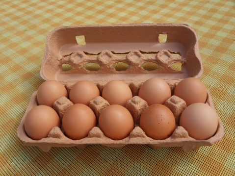
Cartons of Eggs

I’m sure many of you have a carton of eggs in your fridge. Go get me the 17th egg from your carton of eggs. Some of you will be able to do this, and some of you will not. Maybe you only have a 12 egg carton. Maybe you only have 4 eggs in your 18 egg carton, and the 17th egg is one of the ones that are missing. Maybe you’re vegan.

A basic sort of construct in programming is called an “array.” Basically, this is a collection of the same sort of things packed together in a region of memory on your computer. You can think of a carton of eggs as an array of eggs. The carton only contains one sort of thing: an egg. The eggs are all packed together right next to each other with nothing in between. There is some finite amount of eggs.

If I told you “for each egg in the carton, take it out and crack it, and dump it in a bowl starting with the first egg”, you would be able to do this. If I told you “take the 7th egg and throw it at your neighbor’s house” you would be able to do this. In the first example, you would notice when you cracked the last egg. In the second example you would make sure that there was a 7th egg, and if there wasn’t you probably picked some other egg because your neighbor is probably a jerk who deserves to have his house egged. You did this unconsciously because you are a human who can react to dynamic situations. The computer can’t do this.

If you have some array that looks like this (array locations are separated by | bars | and * stars * are outside the array) ***|1|2|3|*** and you told the computer “for each location in the array, add 1 to the number, starting at the first location” it would set the first location to be 2, the second location to be 3, the third location to be 4. Then it would interpret the bits in the location of memory directly to the right of the third location as a number, and it would add 1 to this “number” thereby destroying the data in that location. It would do this forever because this is what you told the machine to do. Suppose that part of memory was involved in controlling the brakes in your 2010 era Toyota vehicle. This is obviously incredibly bad, so how do we prevent this?

The answer is that the programmer (hopefully) knows how big the array is and actually says “starting at location one, for the next 3 locations, add one to the number in the location”. But suppose the programmer messes up, and accidentally says “for the next 4 locations” and costs a multinational company billions of dollars? We could prevent this. There are programming languages that give us ways to prevent these situations. “High level” programming languages such as Java have built-in ways to tell how long an array is. They are also designed to prevent the programmer from telling the machine to write past the end of the array. In Java, the program will successfully write |2|3|4| and then it will crash, rather than corrupting the data outside of the array. This crash will be noticed in testing, and Toyota will save face. We also have “low level” programming languages such as C, which don’t do this. Why do we use low level programming languages? Let’s step through what these languages actually have the machine do for “starting at location one, for the next 3 locations, add one to the number in the location”: First the C program:

NOTE: location[some value] is shorthand for “the location identified by some value.” egg_carton[3] is the third egg in the carton. Additionally, you should read these as sequential instructions “first do this, then do that” Finally, these examples are greatly simplified for the purposes of this article.

1: counter = 1
2: location[counter] = 1 + 1
3: if (counter equals 3) terminate
4: counter = 2
5: location[counter] = 2 + 1
6: if (counter equals 3) terminate
7: counter = 3
8: location[count] = 3 + 1
9: if (counter equals 3) terminate

Very roughly speaking, this is what the computer does. The programmer will use a counter to keep track of their location in the array. After updating each location, they will test the counter to see if they should stop. If they keep going they will repeat this process until the stop condition is satisfied. The Java programmer would write mostly the same program, but the program that translates the Java code into machine code (called a compiler) will add some stuff:

1: counter = 1
2: if (counter greater than array length) crash
3: location[counter] = 1 + 1
4: if (counter equals 3) terminate
5: counter = 2
6: if (counter greater than array length) crash
7: location[counter] = 2 + 1
8: if (counter equals 3) terminate
9: counter = 3
10: if (counter greater than array length) crash
11: location[count] = 3 + 1
12: if (counter equals 3) terminate

As you can see, 3 extra lines were added. If you know for a fact that the array you are working with has a length that is greater than or equal to three, then this code is redundant.

For such a small array, this might not be a huge deal, but suppose the array was a billion elements. Suddenly an extra billion instructions were added. Your phone’s processor likely runs at 1-3 gigahertz, which means that it has an internal clock that ticks 1-3 billion times per second. The smallest amount of time that an instruction can take is one clock cycle, which means that in the best case scenario, the java program takes one entire second longer to complete. The fact of the matter is that “if (counter greater than array length) crash” definitely takes longer than one clock cycle to complete. For a game on your phone, this extra second may be acceptable. For the onboard computer in your car, it is definitely not. Imagine if your brakes took an extra second to engage after you push the pedal? Congressmen would get involved!

In Java, reading off the end of an array is defined. The language defines that if you attempt to do this, the program will crash (it actually does something similar but not the same, but this is outside the scope of this article). In order to enforce this definition, it inserts these extra instructions into the program that implement the functionality. In C, reading off the end of an array is undefined. Since C doesn’t care what happens when you read off the end of an array, it doesn’t add any code to your program. C assume you know what you’re doing, and have taken the necessary steps to ensure your program is correct. The result is that the C program is much faster than the Java program.

There are many such undefined behaviors in programming. For instance, your computer’s division function is partial just like the mathematical version. Java will test that the denominator isn’t zero, and crash if it is. C happily tells the machine to evaluate 8 / 0. Most processors will actually go into a failure state if you attempt to divide by zero, and most operating systems (such as Windows or Mac OSX) will crash your program to recover from the fault. However, there is no law that says this must happen. I could very well create a processor that sends lions to your house to punish you for trying to divide by zero. I could define x / 0 = 17. The C language committee would be perfectly fine with either solution; they just don’t care. This is why people often call languages such as C “unsafe.” This doesn’t mean that they are bad necessarily, just that their use requires caution. A chainsaw is unsafe, but it is a very powerful tool when used correctly. When used incorrectly, it will slice your face off.

What To Do

So, if defining every behavior is slow, but leaving it undefined is dangerous, what should we do? Well, the fact of the matter is that in most cases, the added overhead of adding these extra instructions is acceptable. In these cases, “safe” languages such as Java are preferred because they ensure program correctness. Some people will still write these sorts of programs in unsafe languages such as C (for instance, my own DMP Photobooth is implemented in C), but strictly speaking there are better options. This is part of the explanation for the phenomenon that “computers get faster every year, but [insert program] is just as slow as ever!” Since the performance of [insert program] we deemed to be “good enough”, this extra processing power is instead being devoted to program correctness. If you’ve ever used older versions of Windows, then you know that your programs not constantly crashing is a Good Thing.

This is fine and good for those programs, but what about the ones that cannot afford this luxury? These other programs fall into a few general categories, two of which we’ll call “real-time” and “big data.” These are buzzwords that you’ve likely heard before, “big data” programs are the programs that actually process one billion element arrays. An example of this sort of software would be software that is run by a financial company. Financial companies have billions of transactions per day, and these transactions need to post as quickly as possible. (suppose you deposit a check, you want those funds to be available as quickly as possible) These companies need all the speed they can get, and all those extra instructions dedicated to totality are holding up the show.

Meanwhile “real-time” applications have operations that absolutely must complete in a set amount of time. Suppose I’m flying a jet, and I push the button to raise a wing flap. That button triggers an operation in the program running on the flight computer, and if that operation doesn’t complete immediately (where “immediately” is some fixed, non-zero-but-really-small amount of time) then that program is not correct. In these cases, the programmer needs to have very precise control over what instructions are produced, and they need to make every instruction count. In these cases, redundant totality checks are a luxury that is not in the budget.

Real-time and big data programs need to be fast, so they are often implemented in unsafe languages, but that does not mean that invoking undefined behavior is OK. If a financial company sets your account balance to be check value / 0, you are not going to have a good day. If your car reads the braking strength from a location off to the right of the braking strength array, you are going to die. So, what do these sorts of programs do?

One very common method, often used in safety-critical software such as a car’s onboard computer is to employ strict coding standards. MISRA C is a set of guidelines for programming in C to help ensure program correctness. Such guidelines instruct the developer on how to program to avoid unsafe behavior. Enforcement of the guidelines is ensured by peer-review, software testing, and Static program analysis.

Static program analysis (or just static analysis) is the process of running a program on a codebase to check it for defects. For MISRA C, there exists tooling to ensure compliance with its guidelines. Static analysis can also be more general. Over the last year or so, I’ve been assisting with a research project at UCSD called Liquid Haskell. Simply put, Liquid Haskell provides the programmer with ways to specify requirements about the inputs and outputs of a piece of code. Liquid Haskell could ensure the correct usage of division by specifying a “precondition” that “the denominator must not equal zero.” (I believe that this actually comes for free if you use Liquid Haskell as part of its basic built-in checks) After specifying the precondition, the tool will check your codebase, find all uses of division, and ensure that you ensured that zero will never be used as the denominator.

It does this by determining where the denominator value came from. If the denominator is some literal (i.e. the number 7, and not some variable a that can take on multiple values), it will examine the literal and ensure it meets the precondition of division. If the number is an input to the current routine, it will ensure the routine has a precondition on that value that it not be zero. If the number is the output from some other routine, it verifies that the the routine that produced the value has, as a “postcondition”, that its result will never be zero. If the check passes for all usages of division, your use of division will be declared safe. If the check fails, it will tell you what usages were unsafe, and you will be able to fix it before your program goes live. The Haskell programming language is very safe to begin with, but a Haskell program verified by Liquid Haskell is practically Fort Knox!

The Human Factor

Humans are imperfect, we make mistakes. However, we make up for it in our ability to respond to dynamic situations. A human would never fail to grab the 259th egg from a 12 egg carton and crack it into a bowl; the human wouldn’t even try. The human can see that there is only 12 eggs without having to be told to do so, and will respond accordingly. Machines do not make mistakes, they do exactly what you tell them to, exactly how you told them to do it. If you tell the machine to grab the 259th egg and crack it into a bowl, it will reach it’s hand down, grab whatever is in the space 258 egg lengths to the right of the first egg, and smash it on the edge of a mixing bowl. You can only hope that nothing valuable was in that spot.

Most people don’t necessarily have a strong intuition for what “undefined behavior” is, but mathematicians and programmers everywhere fight this battle every day.

Pure Functional Memoization

There are many computation problems that resonate through the ages. Important Problems. Problems that merit a capital P.

The Halting Problem…

P versus NP…

The Fibonacci sequence…

The Fibonacci sequence is a super-important computation Problem that has vexed mathematicians for generations. It’s so simple!

fibs 0 = 0
fibs 1 = 1
fibs n = (fibs $ n - 1) + (fibs $ n - 2)

Done! Right? Let’s fire up ghci and find out.

*Fibs> fibs 10
55

… looking good…

*Fibs> fibs 40

… still waiting…

102334155

… Well that sure took an unfortunate amount of time. Let’s try 1000!

*Fibs> fibs 1000
*** Exception: <<You died before this returned>>

To this day, science wonders what fibs(1000) is. Well today we solve this!

Memoization

The traditional way to solve this is to use Memoization. In an imperative language, we’d create an array of size n, and prepopulate arr[0] = 0 and arr[1] = 1. Next we’d loop over 2 to n, and for each we’d set arr[i] = arr[i-1] + arr[i-2].

Unfortunately for us, this is Haskell. What to do… Suppose we had a map of the solutions for 0 to i, we could calculate the solution for i + 1 pretty easily right?

fibsImpl _ 0 = 0
fibsImpl _ 1 = 1
fibsImpl m i = (mo + mt)
   where
      mo = Map.findWithDefault undefined (i - 1) m
      mt = Map.findWithDefault undefined (i - 2) m

We return 0 and 1 for i = 0 and i = 1 as usual. Next we lookup n – 1 and n – 2 from the map and return their sum. This is all pretty standard. But where does the map come from?

It turns out that this is one of those times that laziness is our friend. Consider this code:

fibs' n = let m = fmap (fibsImpl m)
                  (Map.fromList (zip [0..n]
                                     [0..n])) in
   Map.findWithDefault undefined n m

When I first saw this pattern (which I call the Wizard Pattern, because it was clearly invented by a wizard), I was completely baffled. We pass the thing we’re creating into the function that’s creating it? Unthinkable!

It turns out that this is just what we need. Because of laziness, the fmap returns immediately, and m points to an unevaluated thunk. So, for i = 0, and i = 1, fibsImpl will return 0 and 1 respectively, and the map will map 0 -> 0 and 1 -> 1. Next for i = 2, Haskell will attempt to lookup from the map. When it does this, it will be forced to evaluate the result of i = 0 and i = 1, and it will add 2 -> 1 to the map. This will continue all the way through i = n. Finally, this function looks up and returns the value of fibs n in linearish time. (As we all know, Map lookup isn’t constant time, but this is a lot better than the exponential time we had before)

So let’s try it out.

*Fibs> fibs' 1
1
*Fibs> fibs' 10
55
*Fibs> fibs' 40
102334155

… so far so good…

*Fibs> fibs' 100
354224848179261915075
*Fibs> fibs' 1000
43466557686937456435688527675040625802564660517371780402481729089536555417949051890403879840079255169295922593080322634775209689623239873322471161642996440906533187938298969649928516003704476137795166849228875
*Fibs> fibs' 10000
33644764876431783266621612005107543310302148460680063906564769974680081442166662368155595513633734025582065332680836159373734790483865268263040892463056431887354544369559827491606602099884183933864652731300088830269235673613135117579297437854413752130520504347701602264758318906527890855154366159582987279682987510631200575428783453215515103870818298969791613127856265033195487140214287532698187962046936097879900350962302291026368131493195275630227837628441540360584402572114334961180023091208287046088923962328835461505776583271252546093591128203925285393434620904245248929403901706233888991085841065183173360437470737908552631764325733993712871937587746897479926305837065742830161637408969178426378624212835258112820516370298089332099905707920064367426202389783111470054074998459250360633560933883831923386783056136435351892133279732908133732642652633989763922723407882928177953580570993691049175470808931841056146322338217465637321248226383092103297701648054726243842374862411453093812206564914032751086643394517512161526545361333111314042436854805106765843493523836959653428071768775328348234345557366719731392746273629108210679280784718035329131176778924659089938635459327894523777674406192240337638674004021330343297496902028328145933418826817683893072003634795623117103101291953169794607632737589253530772552375943788434504067715555779056450443016640119462580972216729758615026968443146952034614932291105970676243268515992834709891284706740862008587135016260312071903172086094081298321581077282076353186624611278245537208532365305775956430072517744315051539600905168603220349163222640885248852433158051534849622434848299380905070483482449327453732624567755879089187190803662058009594743150052402532709746995318770724376825907419939632265984147498193609285223945039707165443156421328157688908058783183404917434556270520223564846495196112460268313970975069382648706613264507665074611512677522748621598642530711298441182622661057163515069260029861704945425047491378115154139941550671256271197133252763631939606902895650288268608362241082050562430701794976171121233066073310059947366875
*Fibs> fibs' 100000
2597406934722172416615503402127591541488048538651769658472477070395253454351127368626555677283671674475463758722307443211163839947387509103096569738218830449305228763853133492135302679278956701051276578271635608073050532200243233114383986516137827238124777453778337299916214634050054669860390862750996639366409211890125271960172105060300350586894028558103675117658251368377438684936413457338834365158775425371912410500332195991330062204363035213756525421823998690848556374080179251761629391754963458558616300762819916081109836526352995440694284206571046044903805647136346033000520852277707554446794723709030979019014860432846819857961015951001850608264919234587313399150133919932363102301864172536477136266475080133982431231703431452964181790051187957316766834979901682011849907756686456845066287392485603914047605199550066288826345877189410680370091879365001733011710028310473947456256091444932821374855573864080579813028266640270354294412104919995803131876805899186513425175959911520563155337703996941035518275274919959802257507902037798103089922984996304496255814045517000250299764322193462165366210841876745428298261398234478366581588040819003307382939500082132009374715485131027220817305432264866949630987914714362925554252624043999615326979876807510646819068792118299167964409178271868561702918102212679267401362650499784968843680975254700131004574186406448299485872551744746695651879126916993244564817673322257149314967763345846623830333820239702436859478287641875788572910710133700300094229333597292779191409212804901545976262791057055248158884051779418192905216769576608748815567860128818354354292307397810154785701328438612728620176653953444993001980062953893698550072328665131718113588661353747268458543254898113717660519461693791688442534259478126310388952047956594380715301911253964847112638900713362856910155145342332944128435722099628674611942095166100230974070996553190050815866991144544264788287264284501725332048648319457892039984893823636745618220375097348566847433887249049337031633826571760729778891798913667325190623247118037280173921572390822769228077292456662750538337500692607721059361942126892030256744356537800831830637593334502350256972906515285327194367756015666039916404882563967693079290502951488693413799125174856667074717514938979038653338139534684837808612673755438382110844897653836848318258836339917310455850905663846202501463131183108742907729262215943020429159474030610183981685506695026197376150857176119947587572212987205312060791864980361596092339594104118635168854883911918517906151156275293615849000872150192226511785315089251027528045151238603792184692121533829287136924321527332714157478829590260157195485316444794546750285840236000238344790520345108033282013803880708980734832620122795263360677366987578332625485944906021917368867786241120562109836985019729017715780112040458649153935115783499546100636635745448508241888279067531359950519206222976015376529797308588164873117308237059828489404487403932053592935976454165560795472477862029969232956138971989467942218727360512336559521133108778758228879597580320459608479024506385194174312616377510459921102486879496341706862092908893068525234805692599833377510390101316617812305114571932706629167125446512151746802548190358351688971707570677865618800822034683632101813026232996027599403579997774046244952114531588370357904483293150007246173417355805567832153454341170020258560809166294198637401514569572272836921963229511187762530753402594781448204657460288485500062806934811398276016855584079542162057543557291510641537592939022884356120792643705560062367986544382464373946972471945996555795505838034825597839682776084731530251788951718630722761103630509360074262261717363058613291544024695432904616258691774630578507674937487992329181750163484068813465534370997589353607405172909412697657593295156818624747127636468836551757018353417274662607306510451195762866349922848678780591085118985653555434958761664016447588028633629704046289097067736256584300235314749461233912068632146637087844699210427541569410912246568571204717241133378489816764096924981633421176857150311671040068175303192115415611958042570658693127276213710697472226029655524611053715554532499750843275200199214301910505362996007042963297805103066650638786268157658772683745128976850796366371059380911225428835839194121154773759981301921650952140133306070987313732926518169226845063443954056729812031546392324981793780469103793422169495229100793029949237507299325063050942813902793084134473061411643355614764093104425918481363930542369378976520526456347648318272633371512112030629233889286487949209737847861884868260804647319539200840398308008803869049557419756219293922110825766397681361044490024720948340326796768837621396744075713887292863079821849314343879778088737958896840946143415927131757836511457828935581859902923534388888846587452130838137779443636119762839036894595760120316502279857901545344747352706972851454599861422902737291131463782045516225447535356773622793648545035710208644541208984235038908770223039849380214734809687433336225449150117411751570704561050895274000206380497967960402617818664481248547269630823473377245543390519841308769781276565916764229022948181763075710255793365008152286383634493138089971785087070863632205869018938377766063006066757732427272929247421295265000706646722730009956124191409138984675224955790729398495608750456694217771551107346630456603944136235888443676215273928597072287937355966723924613827468703217858459948257514745406436460997059316120596841560473234396652457231650317792833860590388360417691428732735703986803342604670071717363573091122981306903286137122597937096605775172964528263757434075792282180744352908669606854021718597891166333863858589736209114248432178645039479195424208191626088571069110433994801473013100869848866430721216762473119618190737820766582968280796079482259549036328266578006994856825300536436674822534603705134503603152154296943991866236857638062351209884448741138600171173647632126029961408561925599707566827866778732377419444462275399909291044697716476151118672327238679208133367306181944849396607123345271856520253643621964198782752978813060080313141817069314468221189275784978281094367751540710106350553798003842219045508482239386993296926659221112742698133062300073465628498093636693049446801628553712633412620378491919498600097200836727876650786886306933418995225768314390832484886340318940194161036979843833346608676709431643653538430912157815543512852077720858098902099586449602479491970687230765687109234380719509824814473157813780080639358418756655098501321882852840184981407690738507369535377711880388528935347600930338598691608289335421147722936561907276264603726027239320991187820407067412272258120766729040071924237930330972132364184093956102995971291799828290009539147382437802779051112030954582532888721146170133440385939654047806199333224547317803407340902512130217279595753863158148810392952475410943880555098382627633127606718126171022011356181800775400227516734144169216424973175621363128588281978005788832454534581522434937268133433997710512532081478345067139835038332901313945986481820272322043341930929011907832896569222878337497354301561722829115627329468814853281922100752373626827643152685735493223028018101449649009015529248638338885664893002250974343601200814365153625369199446709711126951966725780061891215440222487564601554632812091945824653557432047644212650790655208208337976071465127508320487165271577472325887275761128357592132553934446289433258105028633583669291828566894736223508250294964065798630809614341696830467595174355313224362664207197608459024263017473392225291248366316428006552870975051997504913009859468071013602336440164400179188610853230764991714372054467823597211760465153200163085336319351589645890681722372812310320271897917951272799656053694032111242846590994556380215461316106267521633805664394318881268199494005537068697621855231858921100963441012933535733918459668197539834284696822889460076352031688922002021931318369757556962061115774305826305535862015637891246031220672933992617378379625150999935403648731423208873977968908908369996292995391977217796533421249291978383751460062054967341662833487341011097770535898066498136011395571584328308713940582535274056081011503907941688079197212933148303072638678631411038443128215994936824342998188719768637604496342597524256886188688978980888315865076262604856465004322896856149255063968811404400429503894245872382233543101078691517328333604779262727765686076177705616874050257743749983775830143856135427273838589774133526949165483929721519554793578923866762502745370104660909382449626626935321303744538892479216161188889702077910448563199514826630802879549546453583866307344423753319712279158861707289652090149848305435983200771326653407290662016775706409690183771201306823245333477966660525325490873601961480378241566071271650383582257289215708209369510995890132859490724306183325755201208090007175022022949742801823445413711916298449914722254196594682221468260644961839254249670903104007581488857971672246322887016438403908463856731164308169537326790303114583680575021119639905615169154708510459700542098571797318015564741406172334145847111268547929892443001391468289103679179216978616582489007322033591376706527676521307143985302760988478056216994659655461379174985659739227379416726495377801992098355427866179123126699374730777730569324430166839333011554515542656864937492128687049121754245967831132969248492466744261999033972825674873460201150442228780466124320183016108232183908654771042398228531316559685688005226571474428823317539456543881928624432662503345388199590085105211383124491861802624432195540433985722841341254409411771722156867086291742124053110620522842986199273629406208834754853645128123279609097213953775360023076765694208219943034648783348544492713539450224591334374664937701655605763384697062918725745426505879414630176639760457474311081556747091652708748125267159913793240527304613693961169892589808311906322510777928562071999459487700611801002296132304588294558440952496611158342804908643860880796440557763691857743754025896855927252514563404385217825890599553954627451385454452916761042969267970893580056234501918571489030418495767400819359973218711957496357095967825171096264752068890806407651445893132870767454169607107931692704285168093413311046353506242209810363216771910420786162184213763938194625697286781413636389620123976910465418956806197323148414224550071617215851321302030684176087215892702098879108938081045903397276547326416916845445627600759561367103584575649094430692452532085003091068783157561519847567569191284784654692558665111557913461272425336083635131342183905177154511228464455136016013513228948543271504760839307556100908786096663870612278690274831819331606701484957163004705262228238406266818448788374548131994380387613830128859885264201992286188208499588640888521352501457615396482647451025902530743172956899636499615707551855837165935367125448515089362904567736630035562457374779100987992499146967224041481601289530944015488942613783140087804311431741858071826185149051138744831358439067228949408258286021650288927228387426432786168690381960530155894459451808735197246008221529343980828254126128257157209350985382800738560472910941184006084485235377833503306861977724501886364070344973366473100602018128792886991861824418453968994777259482169137133647470453172979809245844361129618997595696240971845564020511432589591844724920942930301651488713079802102379065536525154780298059407529440513145807551537794861635879901158192019808879694967187448224156836463534326160242632934761634458163890163805123894184523973421841496889262398489648642093409816681494771155177009562669029850101513537599801272501241971119871526593747484778935488777815192931171431167444773882941064615028751327709474504763922874890662989841540259350834035142035136168819248238998027706666916342133424312054507359388616687691188185776118135771332483965209882085982391298606386822804754362408956522921410859852037330544625953261340234864689275060526893755148403298542086991221052597005628576707702567695300978970046408920009852106980295419699802138053295798159478289934443245491565327845223840551240445208226435420656313310702940722371552770504263482073984454889589248861397657079145414427653584572951329719091947694411910966797474262675590953832039169673494261360032263077428684105040061351052194413778158095005714526846009810352109249040027958050736436961021241137739717164869525493114805040126568351268829598413983222676377804500626507241731757395219796890754825199329259649801627068665658030178877405615167159731927320479376247375505855052839660294566992522173600874081212014209071041937598571721431338017425141582491824710905084715977249417049320254165239323233258851588893337097136310892571531417761978326033750109026284066415801371359356529278088456305951770081443994114674291850360748852366654744869928083230516815711602911836374147958492100860528981469547750812338896943152861021202736747049903930417035171342126923486700566627506229058636911882228903170510305406882096970875545329369434063981297696478031825451642178347347716471058423238594580183052756213910186997604305844068665712346869679456044155742100039179758348979935882751881524675930878928159243492197545387668305684668420775409821781247053354523194797398953320175988640281058825557698004397120538312459428957377696001857497335249965013509368925958021863811725906506436882127156815751021712900765992750370228283963962915973251173418586721023497317765969454283625519371556009143680329311962842546628403142444370648432390374906410811300792848955767243481200090309888457270907750873638873299642555050473812528975962934822878917619920725138309388288292510416837622758204081918933603653875284116785703720989718832986921927816629675844580174911809119663048187434155067790863948831489241504300476704527971283482211522202837062857314244107823792513645086677566622804977211397140621664116324756784216612961477109018826094677377686406176721484293894976671380122788941309026553511096118347012565197540807095384060916863936906673786627209429434264260402902158317345003727462588992622049877121178405563348492490326003508569099382392777297498413565614830788262363322368380709822346012274241379036473451735925215754757160934270935192901723954921426490691115271523338109124042812102893738488167358953934508930697715522989199698903885883275409044300321986834003470271220020159699371690650330547577095398748580670024491045504890061727189168031394528036165633941571334637222550477547460756055024108764382121688848916940371258901948490685379722244562009483819491532724502276218589169507405794983759821006604481996519360110261576947176202571702048684914616894068404140833587562118319210838005632144562018941505945780025318747471911604840677997765414830622179069330853875129298983009580277554145435058768984944179136535891620098725222049055183554603706533183176716110738009786625247488691476077664470147193074476302411660335671765564874440577990531996271632972009109449249216456030618827772947750764777446452586328919159107444252320082918209518021083700353881330983215894608680127954224752071924134648334963915094813097541433244209299930751481077919002346128122330161799429930618800533414550633932139339646861616416955220216447995417243171165744471364197733204899365074767844149929548073025856442942381787641506492878361767978677158510784235702640213388018875601989234056868423215585628508645525258377010620532224244987990625263484010774322488172558602233302076399933854152015343847725442917895130637050320444917797752370871958277976799686113626532291118629631164685159934660693460557545956063155830033697634000276685151293843638886090828376141157732003527565158745906567025439437931104838571313294490604926582363108949535090082673154497226396648088618041573977888472892174618974189721700770009862449653759012727015227634510874906948012210684952063002519011655963580552429180205586904259685261047412834518466736938580027700252965356366721619883672428226933950325930390994583168665542234654857020875504617520521853721567282679903418135520602999895366470106557900532129541336924472492212436324523042895188461779122338069674233980694887270587503389228395095135209123109258159006960395156367736067109050566299603571876423247920752836160805597697778756476767210521222327184821484446631261487584226092608875764331731023263768864822594691211032367737558122133470556805958008310127481673962019583598023967414489867276845869819376783757167936723213081586191045995058970991064686919463448038574143829629547131372173669836184558144505748676124322451519943362182916191468026091121793001864788050061351603144350076189213441602488091741051232290357179205497927970924502479940842696158818442616163780044759478212240873204124421169199805572649118243661921835714762891425805771871743688000324113008704819373962295017143090098476927237498875938639942530595331607891618810863505982444578942799346514915952884869757488025823353571677864826828051140885429732788197765736966005727700162592404301688659946862983717270595809808730901820120931003430058796552694788049809205484305467611034654748067290674399763612592434637719995843862812391985470202414880076880818848087892391591369463293113276849329777201646641727587259122354784480813433328050087758855264686119576962172239308693795757165821852416204341972383989932734803429262340722338155102209101262949249742423271698842023297303260161790575673111235465890298298313115123607606773968998153812286999642014609852579793691246016346088762321286205634215901479188632194659637483482564291616278532948239313229440231043277288768139550213348266388687453259281587854503890991561949632478855035090289390973718988003999026132015872678637873095678109625311008054489418857983565902063680699643165033912029944327726770869305240718416592070096139286401966725750087012218149733133695809600369751764951350040285926249203398111014953227533621844500744331562434532484217986108346261345897591234839970751854223281677187215956827243245910829019886390369784542622566912542747056097567984857136623679023878478161201477982939080513150258174523773529510165296934562786122241150783587755373348372764439838082000667214740034466322776918936967612878983488942094688102308427036452854504966759697318836044496702853190637396916357980928865719935397723495486787180416401415281489443785036291071517805285857583987711145474240156416477194116391354935466755593592608849200546384685403028080936417250583653368093407225310820844723570226809826951426162451204040711501448747856199922814664565893938488028643822313849852328452360667045805113679663751039248163336173274547275775636810977344539275827560597425160705468689657794530521602315939865780974801515414987097778078705357058008472376892422189750312758527140173117621279898744958406199843913365680297721208751934988504499713914285158032324823021340630312586072624541637765234505522051086318285359658520708173392709566445011404055106579055037417780393351658360904543047721422281816832539613634982525215232257690920254216409657452618066051777901592902884240599998882753691957540116954696152270401280857579766154722192925655963991820948894642657512288766330302133746367449217449351637104725732980832812726468187759356584218383594702792013663907689741738962252575782663990809792647011407580367850599381887184560094695833270775126181282015391041773950918244137561999937819240362469558235924171478702779448443108751901807414110290370706052085162975798361754251041642244867577350756338018895379263183389855955956527857227926155524494739363665533904528656215464288343162282921123290451842212532888101415884061619939195042230059898349966569463580186816717074818823215848647734386780911564660755175385552224428524049468033692299989300783900020690121517740696428573930196910500988278523053797637940257968953295112436166778910585557213381789089945453947915927374958600268237844486872037243488834616856290097850532497036933361942439802882364323553808208003875741710969289725499878566253048867033095150518452126944989251596392079421452606508516052325614861938282489838000815085351564642761700832096483117944401971780149213345335903336672376719229722069970766055482452247416927774637522135201716231722137632445699154022395494158227418930589911746931773776518735850032318014432883916374243795854695691221774098948611515564046609565094538115520921863711518684562543275047870530006998423140180169421109105925493596116719457630962328831271268328501760321771680400249657674186927113215573270049935709942324416387089242427584407651215572676037924765341808984312676941110313165951429479377670698881249643421933287404390485538222160837088907598277390184204138197811025854537088586701450623578513960109987476052535450100439353062072439709976445146790993381448994644609780957731953604938734950026860564555693224229691815630293922487606470873431166384205442489628760213650246991893040112513103835085621908060270866604873585849001704200923929789193938125116798421788115209259130435572321635660895603514383883939018953166274355609970015699780289236362349895374653428746875

Neat. Even that last one only took a few seconds to return!

Baby’s First Proof

Unlike many languages that you learn, in Coq, things are truly different. Much like your first functional language after using nothing but imperative languages, you have to re-evaluate things. Instead of just defining functions, you have to prove properties of them. So, let’s take a look at a few basic ways to do that.

Simpl and Reflexivity

Here we have two basic “tactics” that we can use to prove simple properties. Suppose we have some function addition. We’re all familiar with how this works; 2 + 2 = 4, right? Prove it:

Lemma two_plus_two:
  2 + 2 = 4.
Proof.
  Admitted.

First, what is this Admitted. thing? Admitted basically tells Coq not to worry about it, and just assume it is true. This is the equivalent of your math professor telling you “don’t worry about it, Aristotle says it’s true, are you calling Aristotle a liar?” and if you let this make it into live code, you are a bad person. We must make this right!

Lemma two_plus_two:
  2 + 2 = 4.
Proof.
  simpl.
  reflexivity.
Qed.

That’s better. This is a simple proof; we tell Coq to simplify the expression, then we tell Coq to verify that the left-hand-side is the same as the right-hand-side. One nice feature of Coq is that lets you step through these proofs to see exactly how the evaluation is proceeding. If you’re using Proof General, you can use the buttons Next, Goto, and Undo to accomplish this. If you put the point at Proof. and click Goto, Coq will evaluate the buffer up to that point, and a window should appear at the bottom with the following:

1 subgoals, subgoal 1 (ID 2)

  ============================
   2 + 2 = 4

This is telling you that Coq has 1 thing left to prove: 2 + 2 = 4. Click next, the bottom should change to:

1 subgoals, subgoal 1 (ID 2)

  ============================
   4 = 4

Coq processed the simpl tactic and now the thing it needs to prove is that 4 = 4. Obviously this is true, so if we click next…

No more subgoals.

…reflexivity should succeed, and it does. If we click next one more time:

two_plus_two is defined

This says that this Lemma has been defined, and we can now refer to it in other proofs, much like we can call a function. Now, you may be wondering “do I really have to simplify 2 + 2?” No, you don’t, reflexivity will simplify on it’s own, this typechecks just fine:

Lemma two_plus_two:
  2 + 2 = 4.
Proof.
  reflexivity.
Qed.

So, what’s the point of simpl then? Let’s consider a more complicated proof.

Induction

Lemma n_plus_zero_eq_n:
  forall (n : nat), n + 0 = n.

This lemma state that for any n, n + 0 = n. This is the same as when you’d write ∀ in some math. Other bits of new syntax is n : nat, which means that n has the type nat. The idea here is that no matter what natural number n is, n + 0 = n. So how do we prove this? One might be tempted to try:

Lemma n_plus_zero_eq_n:
  forall (n : nat), n + 0 = n.
Proof.
  reflexivity.
Qed.

One would be wrong. What is Coq stupid? Clearly n + 0 = n, Aristotle told me so! Luckily for us, this is a pretty easy proof, we just need to be explicit about it. We can use induction to prove this. Let me show the whole proof, then we’ll walk through it step by step.

Lemma n_plus_zero_eq_n:
  forall (n : nat), n + 0 = n.
Proof.
  intros n.
  induction n as [| n'].
  {
    reflexivity.
  }
  {
    simpl.
    rewrite -> IHn'.
    reflexivity.
  }
Qed.

Place the point at Proof and you’ll see the starting goal:

1 subgoals, subgoal 1 (ID 6)

  ============================
   forall n : nat, n + 0 = n

Click next and step over intros n.

1 subgoals, subgoal 1 (ID 7)

  n : nat
  ============================
   n + 0 = n

What happened here is intros n introduces the variable n, and names it n. We could have done intros theNumber and the bottom window would instead show:

1 subgoals, subgoal 1 (ID 7)

  theNumber : nat
  ============================
   theNumber + 0 = theNumber

The intros tactic reads from left to right, so if we had some Lemma foo : forall (n m : nat), [stuff], we could do intros nName mName., and it would read in n, and bind it to nName, and then read in m and bind it to mName. Click next and evaluate induction n as [| n'].

2 subgoals, subgoal 1 (ID 10)

  ============================
   0 + 0 = 0

subgoal 2 (ID 13) is:
 S n' + 0 = S n'

The induction tactic implements the standard proof by induction, splitting our goal into two goals: the base case and the n + 1 case. Similarly to intros, this will create subgoals starting with the first constructor of an ADT, and ending with the last.

On Natural Numbers in Coq

Let us take a second to talk about how numbers are represented in Coq. Coq re-implements all types within itself, so nat isn’t a machine integer, it’s an algebraic datatype of the form:

Inductive nat : Set :=
  | O : nat
  | S : nat -> nat.

O is zero, S O is one, and S (S (S (O))) is three. There is a lot of syntax sugar in place that lets you write 49 instead of S (S ( ... ( S O) ... )), and that’s a good thing.

The point of all of this is that we can pattern match on nat much like we can a list.

More Induction

…anyways, all this brings us back to induction and this mysterious as [| n']. What this is doing is binding names to all the fields of the ADT we are deconstructing. The O constructor takes no parameters, so there is nothing to the left of the |. The S constructor takes a nat, so we give it the name n'. Click next and observe the bottom change:

1 focused subgoals (unfocused: 1)
, subgoal 1 (ID 10)

  ============================
   0 + 0 = 0

The curly braces “focuses” the current subgoal, hiding all irrelevant information. Curly braces are optional, but I find them to be very helpful as the bottom window can become very cluttered in large proofs. Here we see the base case goal being to prove that 0 + 0 = 0. Obviously this is true, and we can have Coq verify this by reflexivity. Click next until the next opening curly brace is evaluated. We see the next subgoal:

1 focused subgoals (unfocused: 0)
, subgoal 1 (ID 13)

  n' : nat
  IHn' : n' + 0 = n'
  ============================
   S n' + 0 = S n'

So, what do we have here? This is the n + 1 case; here the n’ in S n' is the original n. A particularly bored reader may try to prove forall (n : nat), S n = n + 1 and I’ll leave that as an exercise. However, this follows from the definition of nat.

Also of note here is IHn'. IH stands for induction hypothesis, and this is that n’ + 0 = n’. So, how do we proceed? Click next and observe how the subgoal changes:

1 focused subgoals (unfocused: 0)
, subgoal 1 (ID 15)

  n' : nat
  IHn' : n' + 0 = n'
  ============================
   S (n' + 0) = S n'

It brought the + 0 inside the S constructor. Notice that now there is n' + 0 on the left hand side. Click next and watch closely what happens:

1 focused subgoals (unfocused: 0)
, subgoal 1 (ID 16)

  n' : nat
  IHn' : n' + 0 = n'
  ============================
   S n' = S n'

Here we use the induction hypothesis to rewrite all occurrences of n' + 0, which was the left hand side of the induction hypothesis as n', which was the right hand side of the induction hypothesis. This is what the rewrite tactic does. Notice now that the subgoal is S n' = S n' which reflexivity will surely find to be true. So, what would happen if we had done rewrite <- IHn'.?

1 focused subgoals (unfocused: 0)
, subgoal 1 (ID 16)

  n' : nat
  IHn' : n' + 0 = n'
  ============================
   S (n' + 0 + 0) = S (n' + 0)

It rewrote all instances of n', which was the right hand side of the induction hypothesis with n' + 0 which was the left hand side of the induction hypothesis. Obviously, this isn’t what we want. I should note that you can undo this by rewriting to the right twice…

  {
    simpl.
    rewrite <- IHn'.
    rewrite -> IHn'.
    rewrite -> IHn'.
    reflexivity.
  }

…and it will technically work. But don’t do this, it’s silly and there’s no room for silliness in a rigorous mathematical proof.

Personally, I have a hard time keeping it straight what the left and right rewrites do. I sometimes find myself just trying one, and then the other if I guessed wrong. Think of it like this: rewrite -> foo rewrites the current goal, replacing all occurrences of the thing on the left hand side of the equation of foo with the thing on the right hand side of the equation. It changes from the left to the right. And vice-versa for rewrite <-, which changes from the right to the left.

Getting Started With Coq and Proof General

Today we’ll be talking about Coq. Coq is a dependently typed programming language and theorem proof assistant. Given that I’ve just now got the toolchain installed, I’m hardly qualified to say much more than that. However, I am qualified to talk about installing the toolchain, which is precisely what I intend to do.

To get started with Coq, you’ll need the usual things: a properly configured editor and the Coq compiler. Installing these isn’t terribly difficult. First, let’s install the compiler. If you’re running Ubuntu, this is quite simple:

$ sudo apt-get install coq

After this is done, you should have access to the compiler (coqc) and the REPL (coqtop):

$ which coqc
/usr/bin/coqc
$ which coqtop
/usr/bin/coqtop
$ coqc --version
The Coq Proof Assistant, version 8.4pl4 (July 2014)
compiled on Jul 27 2014 23:12:44 with OCaml 4.01.0

OK! Now for the (slightly) harder part: our properly configured editor. Here we have two choices: CoqIDE or Proof General. CoqIDE is a simple IDE that ships with Coq, so if you’re satisfied with this, then feel free to stop reading now: CoqIDE comes with Coq and should be already installed at this point!

However, if you want to be truly cool, you’ll opt for Proof General. Proof General is an Emacs plugin. Unfortunately, Proof General is not available in Melpa, so we get to install it manually. Fortunately for us, Proof General is in the repos, so if you’re running Ubuntu you can just apt-get it:

$ sudo apt-get install proofgeneral proofgeneral-doc

This will install Proof General, and set Emacs to load it up when you open a .v file. (My condolences to all those who write Verilog and Coq on the same machine) However, some configuration remains to be done. First fire up emacs and execute:

M-x customize-group <enter> proof-general <enter>

Expand Proof Assistants and ensure Coq is selected. Now open up a .v file and behold the glory!

Wait a minute, where’s my undo-tree? My rainbow-delimiters? My whitespace-mode? It’s not your imagination, Proof General has inexplicably ignored your fancy .emacs config. This is all a bit irritating, but you can work around it by re-adding these things to the coq-mode-hook:

(add-hook 'coq-mode-hook 'rainbow-delimiters-mode)
(add-hook 'coq-mode-hook 'whitespace-mode)
(add-hook 'coq-mode-hook 'undo-tree-mode)

This is a bit of a sorry state of affairs, and if anybody reading this knows a better way I’d love to hear it. For now, I got my shinies back, so it’ll do.

Regardless, Proof General should be ready to go at this point. We are ready to continue our journey down the rabbit hole into wonderland… See you all on the other side!

Demystifying Turing Reductions

Among the many computation theory topics that seem completely inexplicable are Turing Reductions. The basic idea here is that there are certain problems that have been proven to be unsolvable. Given that these problems exist, we can prove other prove that other problems are unsolvable by reducing these problems to a known unsolvable problem.

Turing Machines?

A Turing Machine is a theoretical device. It has an infinitely long tape, divided up into cells. Each cell has a symbol written on it. The Turing Machine can do a few things with this tape: it can read from a cell, write to a cell, move the tape one cell to the left, or move the tape one cell to the right. If the Turing Machine tries to move the cursor off the left side of the tape, the head won’t move. Additionally, the Turing Machine can halt and accept or reject. A Turing Machine has a starting configuration: the tape head begins on the leftmost end of the tape, and the tape has an input written on it.

What the Turing Machine does is implementation specific; one Turing Machine may accept a different input than another. This implementation has a mathematical definition, but we care about the high level definition, that looks similar to this:

M = "On input w:
   1. Read the first cell.
   2. If the cell is not blank, accept
   3. If the cell is blank, output "Was empty"
      onto the tape then reject"

This Turing Machine will accept if there is something written on the tape. If the tape is initially empty, it will write “Was empty” onto the tape and reject. This Turing Machine is a decider because it always halts (I.E. has no infinite loop). We say that the Language of M is the set of all non-empty strings, as it accepts all inputs except the empty string. As you can see, this looks very much like a function written in a programming language. I could implement this in Haskell:

m :: String -> (String, Bool)
m "" = ("Was empty", False)
m w = (w, True)

Consider the following Turing Machine:

M = "On input w:
   1. Move the head to the leftmost tape cell.
   2. Read from the cell
   3. If the cell is blank, accept
   4. If the cell is not blank, move the head one cell to 
      the right
   5. Go to step 2"

This Turing Machine will accept all inputs including the empty string. It’s language is the set of all strings. In Haskell, this might look like this:

m :: String -> Bool
m "" = True
m (c:w) = m w

Spot the bug? What happens if we call this on an infinite list?

m ['a'..]

That’s right, infinite recursion. Despite the bad implementation, this is still a valid Turing Machine. We call this a recognizer. It halts on all inputs that are in the language, and it either halts and rejects, or doesn’t halt on all inputs not in the langauge. A language is decidable if there is a decider for it.

Decidability is Undecidable

Much like higher-order functions in programming, Turing Machines can be used as the input to other Turing Machines. Take the following:

A_TM = "On input <M, w> =
   1. If M is not the encoding of a Turing Machine, reject
   2. Simulate M on w, if M accepts w accept. If M rejects
      w, reject

This very simple Turing Machine accepts the encoding of a Turing Machine, and a string, and if the types are right, returns the result of running the machine on the string. In Haskell:

aTM :: (String -> (String, Bool)) 
       -> String -> (String, Bool)
aTM m w = m w

Seems straight-forward enough; A_TM takes a Turing Machine, and a string and runs them. This is a recognizer because all Turing Machines are at least recognizers, but is it a decider? To figure that out, we need some more tooling.

Much like in programming, if function a calls function b, and b might infinitely loop, then a can also infinitely loop. But let’s suppose we have a function that can take a function as an argument, and get its result, that is guaranteed to never infinitely loop:

alwaysReturns :: (String -> (String, Bool)) 
                 -> String -> (String, Bool)
alwaysReturns f arg = -- Magic

It doesn’t matter how this function is implemented, it just magically can get the result of calling f with arg and it will return the correct result 100% of the time, without running it. We can think of it as some perfect static analysis tool. What a world, right? Now suppose I wrote the following function:

negate :: (String -> (String, Bool)) -> (String, Bool)
negate f = (result, (not accRej))
   where
      (result, accRej) = alwaysReturns f (show f)

Ignoring the fact that functions don’t have Show instances, let’s see what’s going on there. The function negate takes a function as an argument, and calls alwaysReturns on the function, and with show‘d function as its argument. negate then negates the accept/reject result and returns the opposite. In other words, if alwaysReturns f (show f) returns (result, True), then negate returns (result, False). This function will never infinitely loop thanks to alwaysReturns. So, what happens if I do this?

negate negate

Let’s follow the logic: negate delegates to alwaysReturns, which does stuff, then returns the result of negate negate. Next negate returns the opposite of what alwaysReturns said it would. Thus, alwaysReturns did not correctly determine the output of negate. Because of this example, we can definitively know that a function that always correctly decides another function can’t exist. Thus there is at least one Turing Machine that is not decidable, and A_TM cannot be a decider.

So, How About Those Reductions?

Now that we have that all out of the way, let’s talk reductions. It was a bit convoluted, but we’ve proven that the decidability of Turing Machines is undecidable. How can we use this? It turns out that we can use this to prove other problems undecidable. Let’s use my Turing Machines as functions idea to talk about some other undecidable problems.

If a TM Halts is Undecidable

Suppose we had the following function:

alwaysHalts :: (String -> (String, Bool)) -> Bool
alwaysHalts f = -- Magic

This function returns True if the passed-in function will never infinitely loop. If this function existed, then we could implement a function to decide any Turing Machine:

perfectDecider :: (String -> (String, Bool)) 
                  -> String -> (String, Bool))
perfectDecider f w
   | alwaysHalts w = f w
   | otherwise = (w, False)

This function first tests to see if it’s safe to call f, and if so, returns f w. If it’s not safe to call f, it just returns (w, False). However, we already proved that this function couldn’t exist, so the thing that makes it possible must also be impossible.

Suppose we had a Turing Machine R that is an implementation of alwaysHalts, that accepts all Turing Machines over <M, w> that halt. The Turing Machine language implementation of perfectDecider would look like this:

M = "On input <M, w>:
   1. Simulate TM R on <M, w>, if R rejects, reject
   2. Simulate M on w. If M accepts, accept.
      If M rejects, reject

As you can see, the logic is similar. We run R on <M, w>. If R rejects, that means that M didn’t halt, so we reject. Otherwise we return the result of running M on w.

If the Language of a TM is empty is undecidable

Suppose we had the following function:

lIsEmpty :: (String -> (String, Bool)) -> Bool
lIsEmpty f = -- Magic

This function will return True if the language of the provided function is empty, and False if not. Similar to the halting problem above, we want to implement perfectDecider. But how would we do that?

perfectDecider :: (String -> (String, Bool)) 
                  -> String -> (String, Bool))
perfectDecider f w = not (lIsEmpty emptyAsReject)
   where
      emptyAsReject w' =
         if (w' == w)
         then f w'
         else False

So, what’s going on here? We have a function that can decide if the language of a TM is empty. So if we want to construct a decider using this, we need to exploit this property. We write a closure that has this property. The function emptyAsReject rejects any string that does not equal w automatically. Then, it runs f w'. Thus, if f rejects w', then the language of emptyAsReject is empty. otherwise it contains the single string w. Thus we treat the empty set as False, and anything else as True.

We can use this method to prove any arbitrary problem undecidable.

{<M> | M is a Turing Machine, and the language of M is {“happy”, “time”, “gatitos”}} is undecidable

In the culmination of this long-winded post, we’ll prove that it is undecidable if a Turing Machine’s language is {“happy”, “time”, “gatitos”}. As before, we’ll assume we have the following function:

lIsHappyTimeGatitos :: (String -> (String, Bool)) -> Bool
lIsHappyTimeGatitos f = -- Magic

We’ll use this to solve the ultimate problem in computer science!

perfectDecider :: (String -> (String, Bool)) 
                  -> String -> (String, Bool))
perfectDecider f w = lIsHappyTimeGatitos hgtAsAccept
   where
      hgtAsAccept "happy" = True
      hgtAsAccept "time" = True
      hgtAsAccept "gatitos" = f w
      hgtAsAccept _ = False

Here, we construct a closure that has the desired property language if f accepts w, and does not have the desired language if f rejects w. hgtAsAccept always accepts “happy” and “time”, but only accepts “gatitos” if f w == True. Thus, if f does not accept w, then lIsHappyTimeGatitos will reject hgtAsAccept, and vice versa.

Well, When You Put It That Way…

Math is nice and all, but we’re programmers. I feel that this is a concept that is not that hard, but when math runes get involved, things get difficult. I think you can see how this works, and grasp the concept. Thinking of these reductions as functions helped me, and I hope it helps you too.

Doing My Math Homework…

Well, it was bound to happen some day… Recently, a new quarter began, and with it new classes. One of said classes is a boolean algebra class, which means lots of fancy math runes to be drawn on pieces of dead trees. One problem though; homework in this class needs to be submitted as a .pdf online. Crap.

I’ve written about this sort of thing before, however, I also remember that being a gigantic hassle. Not to mention the fact that boolean algebra involves drawing logic gates, which is outside the scope of that. I decided it was high time I get onboard the LaTex train.

One Problem…

What problem? Learning LaTeX sounds like a huge hassle. I have enough problems without spending God knows how long learning a new markup language just to submit what would take 20 minutes to write on a piece of paper. In short: I don’t got time for that! Luckily for us, we have tools for this sort of thing.

Last month I wrote about giving Emacs a shot. So far, things have been going well. In fact, one tool that Emacs is known for, org-mode, is actually suited particularly well for this problem. I’ll spare you the basics, and just link to the excellent David O'Toole Org tutorial. If you are unfamiliar with org-mode, I suggest you go give it a read before continuing here.

…back? Good. Among the many things that org-mode is good for, it can be used to produce different kinds of output. Among them are html and our good friend LaTeX.

Document Structure

Let me assign some homework to myself, and we’ll work through it!

Show that AB + B'C + AC = AB + B'C without
directly applying the Consensus Theorem

As you can imagine, AB + B’C + AC = AB + B’C because some fancy Consensus Theorem says so. Our task is to do stuff until the left-hand-side turns into the right-hand-side. And to do it in LaTeX!

First, we need to set up our document structure. Create a new file called homework.org, and create a heading:

* Show using boolean algebra:

This will create a new heading. Now, we need to do some boilerplate first. Add the following to the top of your file:

#+OPTIONS: toc:nil

This will prevent org-mode from creating a table of contents for your homework. I think a table of contents is silly for something with only a few pages, but it sure looks neat! Next, our equations will be automatically numbered, but we want them numbered by section. Add the following below the options line:

\numberwithin{equation}{section}

Now, let’s do some LaTeX. org-mode allows us to do inline LaTeX, and it will use it in the final document. Let’s add an equation block:

* Show using boolean algebra:

  \begin{equation}
  AB + \overline{B}C + AC = AB + \overline{B}C
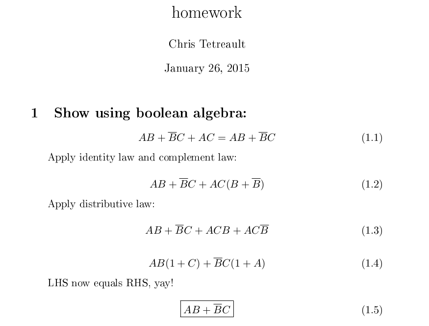
  \end{equation}

If you save, then press: C-c C-e, then l o, your default .pdf reader should launch with a fancy new page that looks something like this:

Let’s do some more math! You can write comments inside of your heading, and they will be part of that section:

  Apply identity law and complement law:

  \begin{equation}
  AB + \overline{B}C + AC(B + \overline{B})
  \end{equation}

  Apply distributive law:

  \begin{equation}
  AB + \overline{B}C + ACB + AC\overline{B}
  \end{equation}

Re-export your new document and you should see something like this:

You may have noticed that we are basically done. Let’s write our answer down along with a fancy box so the professor knows it’s the answer:

  \begin{equation}
  \boxed{AB + \overline{B}C}
  \end{equation}

And we’re done! If you export your document you should see:

I thought you didn’t want to learn LaTex…

I know, there’s a whole lot of LaTeX in there. But it could be worse, let’s take a look at the source file that org-mode creates:

% Created 2015-01-26 Mon 18:26
\documentclass[11pt]{article}
\usepackage[utf8]{inputenc}
\usepackage[T1]{fontenc}
\usepackage{fixltx2e}
\usepackage{graphicx}
\usepackage{longtable}
\usepackage{float}
\usepackage{wrapfig}
\usepackage{rotating}
\usepackage[normalem]{ulem}
\usepackage{amsmath}
\usepackage{textcomp}
\usepackage{marvosym}
\usepackage{wasysym}
\usepackage{amssymb}
\usepackage{hyperref}
\tolerance=1000
\author{Chris Tetreault}
\date{\today}
\title{homework}
\hypersetup{
  pdfkeywords={},
  pdfsubject={},
  pdfcreator={Emacs 24.3.1 (Org mode 8.2.10)}}
\begin{document}

\maketitle
\numberwithin{equation}{section}

\section{Show using boolean algebra:}
\label{sec-1}

\begin{equation}
AB + \overline{B}C + AC = AB + \overline{B}C
\end{equation}

Apply identity law and complement law:

\begin{equation}
AB + \overline{B}C + AC(B + \overline{B})
\end{equation}

Apply distributive law:

\begin{equation}
AB + \overline{B}C + ACB + AC\overline{B}
\end{equation}

\begin{equation}
AB(1 + C) + \overline{B}C(1 + A)
\end{equation}

LHS now equals RHS, yay!

\begin{equation}
\boxed{AB + \overline{B}C}
\end{equation}
% Emacs 24.3.1 (Org mode 8.2.10)
\end{document}

Yeah… Doesn’t seem so bad now. Thanks to org-mode, we can use just enough LaTeX to do what we need to do, and not have to worry about all that boilerplate!

K&R Challenge 3 and 4: Functional Temperature Conversion

The other day, I implemented the C solution to exercises 3 and 4 in The C Programming Language, today I’ll be implementing the Haskell solution. As a reminder, the requirements are:

Modify the temperature conversion program to print a heading above the table

… and …

Write a program to print the corresponding Celsius to Fahrenheit table.

I could take the easy way out, and implement the Haskell solution almost identically to the C solution, replacing the for loop with a call to map, but that’s neither interesting to do, nor is it interesting to read about. I’ll be taking this problem to the next level.

Requirements

For my temperature program, I’d like it to be able to convert between any arbitrary temperature unit. For the purposes of this post, I will be implementing Celsius, Fahrenheit, Kelvin (equivalent to Celsius, except 0 degrees is absolute zero, not the freezing point of water), and Rankine (the Fahrenheit version of Kelvin).

That said, nothing about my solution should rely on the fact that these four temperature scales are being implemented. A programmer should be able to implement a new temperature unit with minimal changes to the program. Ideally, just by implementing a new type.

Additionally, given a bunch of conversions, the program should be able to output a pretty table showing any number of temperature types and indicating what converts to what.

First, Conversion

This problem is clearly broken up into two sub-problems: conversion, and the table. First, we need to handle conversion. This being Haskell, the right answer is likely to start by defining some types. Let’s create types for our units:

newtype Celsius = Celsius Double deriving (Show)
newtype Fahrenheit = Fahrenheit Double deriving (Show)
newtype Kelvin = Kelvin Double deriving (Show)
newtype Rankine = Rankine Double deriving (Show)

I’ve chosen to make a type for each unit, and since they only contain one constructor with one field, I use a newtype instead of a data. Now, how to convert these? A straightforward solution to this would be to define functions that convert each type to each other type. Functions that look like:

celsiusToFahrenheit :: Celsius -> Fahrenheit
celsiusToKelvin :: Celsius -> Kelvin

...

rankineToKelvin :: Rankine -> Kelvin
rankineToCelsius :: Rankine -> Celsius

A diagram for these conversions looks like this:

That’s a lot of conversions! One might argue that it’s manageable, but it certainly doesn’t meet requirement #1 that implementing a new unit would require minimal work; to implement a new conversion, you’d need to define many conversion functions as well! There must be a better way.

Let’s think back to chemistry class. You’re tasked with converting litres to hours or somesuch. Did you do that in one operation? No, you used a bunch of intermediate conversion to get to what you needed. If you know that X litres are Y dollars, and Z dollars is one 1 hour, then you know how many litres are in 1 hour! These are called conversion factors.

Luckily for us, our conversions are much simpler. For any temperature unit, if we can convert it to and from celsius, then we can convert it to and from any other unit! Let’s define a typeclass for Temperature:

class Temperature a where
   toCelsius :: a ->
                Celsius
   fromCelsius :: Celsius ->
                  a
   value :: a ->
            Double
   scaleName :: a ->
                String
   convert :: (Temperature b) =>
              a -> 
              b
   convert f = fromCelsius $ toCelsius f

Our Temperature typeclass has five functions: functions to convert to and from celsius, a function to get the value from a unit, a function to get the name of a unit, and a final function convert. This final function has a default implementation that converts a unit to celsius, then from celsius. Using the type inferrer, this will convert any unit to any other unit!

convert Rankine 811 :: Kelvin
convert Celsius 123 :: Fahrenheit
convert Kelvin 10000 :: RelativeToHeck

Now to implement a new temperature, you only need to implement four functions, as convert is a sane solution for all cases. This arrangement gives us a conversion diagram that looks like:

Much better. Let’s go through our Temperature implementations for our types:

instance Temperature Celsius where
   toCelsius c = c
   fromCelsius c = c
   value (Celsius c) = c
   scaleName _ = "Celsius"

Of course Celsius itself has to implement Temperature. It’s implementation is trivial though; no work needs to be done.

instance Temperature Fahrenheit where
   toCelsius (Fahrenheit f) = Celsius ((5 / 9) * (f - 32))
   fromCelsius (Celsius c) = Fahrenheit ((9 / 5) * c + 32)
   value (Fahrenheit f) = f
   scaleName _ = "Fahrenheit"

Now things are heating up. The conversion functions are identical to the C implementation.

instance Temperature Kelvin where
   toCelsius (Kelvin k) = Celsius (k - 273.15)
   fromCelsius (Celsius c) = Kelvin (c + 273.15)
   value (Kelvin k) = k
   scaleName _ = "Kelvin"

The Kelvin implementation looks much like the Fahrenheit one.

instance Temperature Rankine where
   toCelsius (Rankine r) = toCelsius $ Fahrenheit (r - 459.67)
   fromCelsius c = Rankine $ 459.67 + value (fromCelsius c :: Fahrenheit)
   value (Rankine r) = r
   scaleName _ = "Rankine"

The conversion between Fahrenheit and Rankine is much simpler than the conversion between Celsius and Rankine; therefore I will do just that. After converting to and from Fahrenheit, it’s a simple matter of calling toCelsius and fromCelsius.

Bringing The Monads

Now that the easy part is done, we get to create the table. Our table should have as many columns as it needs to display an arbitrary number of conversions. To that end, let’s define a data structure or two:

data ConversionTable = ConversionTable [String]
                                       [[TableRowElem]] deriving (Show)

data TableRowElem = From Double | To Double
                                | NullConv Double
                                | Empty deriving (Show)

The ConverstionTable, like the name suggests, is our table. The list of strings is the header, and the list of lists of TableRowElem are our conversions. Why not just have a list of Double? We need to have our cells contain information on what they mean.

To that end, I created a TableRowElem type. From is an original value, To is a converted value, NullConv represents the case were we convert from some type to the same type, and Empty is an empty cell. The problem of how to place elements into this data structure still remains however. To solve that, things are going to get a bit monadic. Let’s define some intermediate builder types:

type Conversion a b = (a, b)

toConversion :: (Temperature a, Temperature b) =>
                a ->
                (a, b)
toConversion a = (a, convert a)

First we have Conversion, and the corresponding toConversion function. This simply takes a unit, and places it in a tuple with its corresponding conversion. Next, we have the TableBuilder:

type TableBuilder a = WriterT [[TableRowElem]]
                              (State [String]) a

Here we have a WriterT stacked on top of a State monad. The writer transformer contains the list of table rows, and the state monad contains the header. The idea is that as rows are “logged” into the writer, the header is checked to make sure no new units were introduced. To this end, if only two units are introduced, the table will have two columns. If 100 units are used, then the table will have 100 columns.

NOTE: I realize that WriterT and State are not in the standard library. I only promised to limit the usage of libraries for Haskell solutions. This means avoiding the use of things like Parsec or Happstack. Frameworks and libraries that vastly simplify some problem or change the way you approach it. To this end, if I feel a monad transformer or anything along these lines are appropriate to a problem, I will use them. I’ll try to point out when I do though. Besides, I could have just re-implemented these things, but in the interest of not being a bad person and re-inventing the wheel, I’ve decided to use a wheel off the shelf.

So, how do we use this TableBuilder? I’ve defined a function for use with this monad:

insertConv :: (Temperature a, Temperature b) =>
              Conversion a b ->
              TableBuilder ()
insertConv (a, b) = 
   do oldHeader <- lift $ get
      workingHeader <- ensureElem a oldHeader
      finalHeader <- ensureElem b workingHeader
      lift $ put finalHeader
      tell [buildRow a b finalHeader []]
   where ensureElem a h = return $ case ((scaleName a) `elem` h)
                                        of True -> h
                                           False -> h ++ [(scaleName a)]
         buildRow _ _ [] r = r
         buildRow a b (h:xs) r
            | (scaleName a) == (scaleName b) && (scaleName a) == h = r ++ [NullConv $ value a]
            | (scaleName a) == h = buildRow a b xs (r ++ [From $ value a])
            | (scaleName b) == h = buildRow a b xs (r ++ [To $ value b])
            | otherwise = buildRow a b xs (r ++ [Empty])

Yeah, that one is kind of a doosey. Let me walk you through it. This function takes a Conversion, and returns a TableBuilder.

In the first four lines of the do block, we update the header. We lift the State monad, then get we call ensureElem with the first and second units, then we put the new updated header back into the State monad.

The ensureElem function checks the header list to see if the current unit is a member. If it is, the header list is returned unchanged, if it’s not the unit is appended to the end and the new list is returned. In this way, whenever a conversion is added to the table, the header is updated.

After updating the header, we call tell with the result of buildRow, “writing” the row into the Writer monad. The buildRow function recursively adds TableRowElems to the result list depending on the current heading. In this way, conversions are placed in the appropriate column.

In addition to that function, I’ve defined a function to simplify working with the TableBuilder:

buildTable :: TableBuilder a ->
              ConversionTable
buildTable b = let result = runState (runWriterT b) []
               in ConversionTable (snd result)
                                  (snd $ fst result)

Working with some of these MTL monads can be confusing for people coming from imperative backgrounds. I’ve been working with Haskell for almost a year now and I still get extremely confused by them. It can take some muddling through haddoc pages to work them out, but the good news is that you mainly just need to define one function that takes a monad (in the form of a do block), and returns a whatever. The buildTable function takes a TableBuilder, and returns a ConversionTable. It handles calls to runState and runWriterT, and then unwraps the resulting tuple and builds the ConversionTable.

This function can be called like this:

buildTable $ do insertConv someConversion
                insertConv someOtherConversion

… and so on. The only thing to remember is that the final value of a for the do block must be (). Conveniently, insertConv return a value of type TableBuilder (), so if the last call is to this function, then you are good. You can also always end it with return () if you like.

Pretty Printing

Finally, we have the matter of printing a nice pretty table. For that, we need yet another function:

prettyPrint :: ConversionTable ->
               String
prettyPrint (ConversionTable h r) = let widestCol = last $ sort $ map length h
                                        columnCount = length h
                                        doubleCell = printf ("%-" ++ (show widestCol) ++ ".1f")
                                        stringCell = printf ("| %-" ++ (show widestCol) ++ "s |")
                                        emptyCell = replicate widestCol ' '
                                        horizontalR = (replicate (((widestCol + 4) * columnCount) + 2) '-') ++ "\n"
                                        formatRow row = "|" ++ (concat $ map formatCell row) ++ "|\n"
                                        formatCell (From from) = "| " ++ (doubleCell from) ++ " |"
                                        formatCell (To to) = "> " ++ (doubleCell to) ++ " |"
                                        formatCell Empty = "| " ++ emptyCell ++ " |"
                                        formatCell (NullConv nc) = "| " ++ (doubleCell nc) ++ " |"
                                    in horizontalR
                                          ++ ("|" ++(concat $ map stringCell h) ++ "|\n") 
                                          ++ horizontalR
                                          ++ (concat $ map formatRow (normalizeRowLen (columnCount) r))
                                          ++ horizontalR
            where normalizeRowLen len rows = map (nRL' len) rows
                                  where nRL' len' row
                                           | (length row) < len' = nRL' len' (row ++ [Empty])
                                           | otherwise = row

Yeah… Sometimes the littlest things take the most work. You’d think all this plumbing we’ve been doing would be the most complecated bit, but you’d be wrong. Let’s try to make sense of this mess function by function:

widestCol = last $ sort $ map length h

This function determines the widest column based on the header. Typically, this is going to be “Fahrenheit”, but it doesn’t have to be. It should be noted that if a data cell is wider than this, then the pretty printer will mess up. Like most things in life, there is room for improvement here. That said, unless you’re converting the temperature of the core of the sun, you probably won’t have an issue here.

columnCount = length h

Returns the number of columns in the table. Used by the horizontal rule function.

doubleCell = printf ("%-" ++ (show widestCol) ++ ".1f")

Ahh, our old friend printf. It exists in Haskell and works in much the same way as it did in C. The doubleCell function converts a temperature value to a string, left aligns it, pads it by widestCol, and has it show one decimal place.

stringCell = printf ("| %-" ++ (show widestCol) ++ "s |")

Much like with doubleCell, this function pads, and left-aligns a string. This is used by the header.

emptyCell = replicate widestCol ' '

This one is pretty self-explanatory. It prints an empty cell of the appropriate width.

horizontalR = (replicate (((widestCol + 4) * columnCount) + 2) '-') ++ "\n"

This function prints a horizontal rule. This will be a solid line of “-” across the width of the table.

formatRow row = "|" ++ (concat $ map formatCell row) ++ "|\n"

This function formats a table data row. It maps formatCell over the list of cells, flattens it, then adds a pretty border around it.

formatCell (From from) = "| " ++ (doubleCell from) ++ " |"
formatCell (To to) = "> " ++ (doubleCell to) ++ " |"
formatCell Empty = "| " ++ emptyCell ++ " |"
formatCell (NullConv nc) = "| " ++ (doubleCell nc) ++ " |"

In this function, much of the work is done. It formats the cell using doubleCell or emptyCell, the applies a border to the cell. It denotes a cell containing a To by adding a > on the left.

Now that we’ve covered the let-bound functions, let’s talk about the actual function body:

horizontalR
   concat $ map stringCell h) ++ "|\n") 
   horizontalR
   concat $ map formatRow (normalizeRowLen (columnCount) r))
   horizontalR

This bit is prett straightforward. First, it prints a horizontal line. Second, it maps stringCell over the header list, flattens it, and gives it a border. Third it prints another horizontal line. Fourth is maps formatRow over the normalized row list, then flattens it. Finally, one last horizontal line. After this is all said and done, it concats it all together.

You may be wondering about that normalizeRowLen function. If you were paying particularly close attention to the insertConv function, you may have noticed an issue. Let’s walk through it in ghci:

*Main> let fc = toConversion (Fahrenheit 100) :: (Fahrenheit, Celsius)
*Main> buildTable $ do insertConv fc
ConversionTable ["Fahrenheit","Celsius"] [[From 100.0,To 37.77777777777778]]

We add one conversion, we get two columns. Everything seems to be in order here, but let’s add another conversion and see what happens:

*Main> let fc = toConversion (Fahrenheit 100) :: (Fahrenheit, Celsius)
*Main> let cr = toConversion (Celsius 100) :: (Celsius, Rankine)
*Main> buildTable $ do {insertConv fc; insertConv cr;}
ConversionTable ["Fahrenheit","Celsius","Rankine"] [[From 100.0,To 37.77777777777778],[Empty,From 100.0,To 671.6700000000001]]

See the problem? Let’s add some newlines to make it clearer:

ConversionTable ["Fahrenheit","Celsius","Rankine"]
                [[From 100.0,To 37.77777777777778],
                [Empty,From 100.0,To 671.6700000000001]]

As we add more columns, the rows with less columns are never updated to have the new column count. Logically, this is fine, since the extra entries would just be Empty anyways, but our pretty printer would print this table like so:

--------------------------------------------
|| Fahrenheit || Celsius    || Rankine    ||
--------------------------------------------
|| 100.0      |> 37.8       ||
||            || 100.0      |> 671.7      ||
--------------------------------------------

As you add more and more columns, the problem gets worse and worse. Enter our normalizeRowLen function:

normalizeRowLen len rows = map (nRL' len) rows
                where nRL' len' row
                   | (length row) < len' = nRL' len' (row ++ [Empty])
                   | otherwise = row

This is another fairly straightforward function. If the row has the same number of columns as the header, it is returned unchanged. If it doesn’t, Empty is added to the end until it does.

With that, our program is complete. Let’s try it out:

main = do k <- return (toConversion $ Kelvin 100 :: (Kelvin, Rankine))
          f <- return (toConversion $ Fahrenheit 451 :: (Fahrenheit, Kelvin))
          r <- return (toConversion $ Rankine 234 :: (Rankine, Celsius))
          c <- return (toConversion $ Celsius 9 :: (Celsius, Fahrenheit))
          nc <- return (toConversion $ Rankine 123 :: (Rankine, Rankine))
          
          putStrLn $ prettyPrint $ buildTable $ do insertConv k
                                                   insertConv f
                                                   insertConv r
                                                   insertConv c
                                                   insertConv nc

In our main, we create a bunch of conversions. Then we prettyPrint them and putStrLn the result. The following will be printed to the console:

----------------------------------------------------------
|| Kelvin     || Rankine    || Fahrenheit || Celsius    ||
----------------------------------------------------------
|| 100.0      |> 180.0      ||            ||            ||
|> 505.9      ||            || 451.0      ||            ||
||            || 234.0      ||            |> -143.2     ||
||            ||            |> 48.2       || 9.0        ||
||            || 123.0      ||            ||            ||
----------------------------------------------------------

Any type that implements Temperature can be put into a table this way. To add a new unit to the program, it’s as easy as implementing four one-line functions!

K&R Challenge 3 and 4: Fiddling With Formatting Strings

Today I’ll be doing things a bit differently. Since exercise 3 and 4 are quite trivial, and because the Haskell implementation will differ significantly from the C solution, I’m going to break them up into separate posts. In this post, I will implement the C solution to problems 3 and 4, and another day I’ll implement the Haskell solution.

The problem for exercise 3 is:

Modify the temperature conversion program to print a heading above the table

The program in question is as follows:

int main (int argc, char ** argv)
{
   float fahr, celsius;
   int lower, upper, step;
   
   lower = 0;
   upper = 300;
   step = 20;
   
   fahr = lower;
   
   while (fahr <= upper)
   {
      celsius = (5.0/9.0) * (fahr-32.0);
      printf("%3.0f %6.1f\n", fahr, celsius);
      fahr = fahr + step;
   }
   return 0;
}

If compiled and executed, this will print the following:

  0  -17.8
 20   -6.7
 40    4.4

   ...

280  137.8
300  148.9

Strictly speaking, this is a trivial problem. The solution is to add the following line before the while loop:

printf("F     C\n");

Now, we have our header:

F     C
  0  -17.8
 20   -6.7

   ...

280  137.8
300  148.9

Problem 4 is as follows:

Write a program to print the corresponding Celsius to Fahrenheit table.

This can be implemented by simply changing the line…

celsius = (5.0/9.0) * (fahr-32.0)

…to…

fahr = (9.0/5.0) * celsius+32;

…and changing the corresponding printf calls to swap the pairs. Nothing groundbreaking here. Now, let’s talk about my combined solution.

The Solutions

First, we tackle exercise 3. Technically, my previous answer fit the requirements, but I wouldn’t call it “good”. Clearly some pretty printing is in order. Additionally, I’d like to make a table with four columns to print the Fahrenheit to Celsius conversion next to the Celsius to Fahrenheit conversion. To that end, let’s add the following above the loop:

printf("Celsius <- Fahrenheit | Celsius -> Fahrenheit\n");
printf("----------------------|----------------------\n");

This is pretty self-explanatory. We Make some nice pretty columns with a horizontal line between the header and the data. On the left is the Fahrenheit to Celsius conversion, and the right is the Celsius to Fahrenheit conversion. Next, the table.

We’ll need to add extra variables to store the exercise 3 and 4 temperatures. Let’s modify our variables:

float fahr_ex3, celsius_ex3, fahr_ex4, celsius_ex4;

Now we need to calculate both conversions given the same interval:

celsius_ex3 = (5.0/9.0) * (fahr_ex3-32.0);
fahr_ex4 = (9.0/5.0) * celsius_ex4+32;

After that’s done, we need to print the table row we just calculated:

printf("%7.1f <- %-10.1f | %7.1f -> %-10.1f\n", 
             celsius_ex3, 
             fahr_ex3,
             celsius_ex4,
             fahr_ex4);

Here we’ve updated our printf statement. We now print all four variables on one line. Additionally we’ve updated the formatting options to line the entries up neatly within the columns.

Finally, we need to modify some loop bookkeeping:

fahr_ex3 = lower;
celsius_ex4 = lower;
while (fahr_ex3 <= upper && celsius_ex4 <= upper)
{
   
   /*Do Stuff*/
   
   fahr_ex3 = fahr_ex3 + step;
   celsius_ex4 = celsius_ex4 + step;
}

And we’re done! If you compile and execute this new program, the following should print to the terminal:

Celsius <- Fahrenheit | Celsius -> Fahrenheit
----------------------|----------------------
  -17.8 <- 0.0        |     0.0 -> 32.0
   -6.7 <- 20.0       |    20.0 -> 68.0
    4.4 <- 40.0       |    40.0 -> 104.0
   15.6 <- 60.0       |    60.0 -> 140.0
   26.7 <- 80.0       |    80.0 -> 176.0
   37.8 <- 100.0      |   100.0 -> 212.0
   48.9 <- 120.0      |   120.0 -> 248.0
   60.0 <- 140.0      |   140.0 -> 284.0
   71.1 <- 160.0      |   160.0 -> 320.0
   82.2 <- 180.0      |   180.0 -> 356.0
   93.3 <- 200.0      |   200.0 -> 392.0
  104.4 <- 220.0      |   220.0 -> 428.0
  115.6 <- 240.0      |   240.0 -> 464.0
  126.7 <- 260.0      |   260.0 -> 500.0
  137.8 <- 280.0      |   280.0 -> 536.0
  148.9 <- 300.0      |   300.0 -> 572.0

Aside from just looking nicer, I’d say this is more in line with the spirit of the exercise. After all, when faced with a requirements document, you can either give a customer exactly what they asked for, or you can give them what they actually want. Which is more likely to get sent back for rework?

The complete source for this solution:

#include <stdio.h>
int main (int argc, char ** argv)
{
   float fahr_ex3, celsius_ex3, fahr_ex4, celsius_ex4;
   int lower, upper, step;
   lower = 0;
   upper = 300;
   step = 20;
   fahr_ex3 = lower;
   celsius_ex4 = lower;
   printf("Celsius <- Fahrenheit | Celsius -> Fahrenheit\n");
   printf("----------------------|----------------------\n");
   while (fahr_ex3 <= upper && celsius_ex4 <= upper)
   {
      celsius_ex3 = (5.0/9.0) * (fahr_ex3-32.0);
      fahr_ex4 = (9.0/5.0) * celsius_ex4+32;
      printf("%7.1f <- %-10.1f | %7.1f -> %-10.1f\n", 
             celsius_ex3, 
             fahr_ex3,
             celsius_ex4,
             fahr_ex4);
      fahr_ex3 = fahr_ex3 + step;
      celsius_ex4 = celsius_ex4 + step;
   }
   return 0;
}

UPDATE: The Haskell solution can be found here.

Monads In Clinical Terms

Last week, we briefly discussed Monads. If you haven’t read that post, it would probably be helpful to do so now. To recap, I talked about two things. First and foremost I talked about how monads are horrific and terrifying. Secondly I talked about the use of the bind operator, and do notation in Haskell.

Today I’ll be discussing at a very low level, what exactly a Monad is. I feel that there is a general notion that all Monads are similar to each other, and serve some common purpose. I know this has been causing issues for me. However, I’m slowly coming around to the idea that they really aren’t. Let’s consider some of the monads in Haskell. We have:

• The List monad, which is a data structure.
• The Maybe monad, which represents the result of a calculation that may have failed.
• The Either monad, which represents a value, or an error.

I know what you may be thinking: “These all look like data structures!” I had this same thought, but let’s look at some more monads:

• The IO monad, which represents some communication with the “outside world”.
• The Writer monad, which represents logging.
• The State monad, which represents program state.

…and then that notion falls apart. If you tried really hard, you might make a case that these are all data structures. However, they’re really not. So, what exactly is a monad? At the very basic level, a monad is two functions, and three laws. Let’s take a look at these.

Two Functions

I touched on this a bit last week, but in order for something to be a monad, it must implement two functions: bind and return. Let’s take a look at these.

Bind

Any monad typically contains a value, and some “decoration”. Bind takes a monad, a function that takes a value and returns a monad, calls that function on the value contained in the old monad, returning a new monad. Finally the logic contained within the bind function “reconciles” the old monad and new monad’s decorations, returning the final resulting monad. Conceptually, this looks something like this:

Let’s take a look at Haskell’s bind operator’s function signature:

(>>=) :: m a -> (a -> m b) -> m b

In Haskell, bind is implemented as an operator: >>=. This takes a monad containing an “a“, a function that takes an “a“, and returns a monad containing a “b“, and finally returns a monad containing a “b“. It is up to the author of a monad to determine what it means to “reconcile the decoration” taking into account the laws I’m going to talk about in a minute.

return

Compared to bind, return is child’s play. Simply put, return takes a value, and creates a new monad with the most basic amount of decoration to still be valid. This is functionally equivalent to the pure function provided by Applicative Functors.

Three Laws

While you can make any old thing a member of the Monad typeclass, it’s not actually a monad unless it obeys the law. There are three properties that a monad must satisfy in order to be a valid monad:

Left identity

Formally defined as:

return a >>= k == k a

This law states that calling return on some value, and then binding the resulting monad to some function should have the same result as just calling that function on the value. The idea here is that if return truly gives a value minimal decoration, that this decoration should not change the resulting monad of a function when bound. Let’s see how Maybe satisfies this law. Here is Maybe‘s instance definition:

instance Monad Maybe where
    (Just x) >>= k = k x
    Nothing >>= _ = Nothing
    return k = Just k

When Maybe‘s return implementation is called, it wraps the argument in a Just. Maybe has two bind implementations, one for Just and one for Nothing. If a Just is bound to a function, the function will be called on the value contained in the Just, and the resulting Maybe is the result of the bind function. Therefore, if the function returns a Just, bind returns that Just. If the function returns Nothing, then bind returns that Nothing.

As you can see, return always returns Just k, therefore Maybe satisfies the law of Left Identity.

Right Identity

Formally defined as:

m >>= return  ==  m

return is a function that takes a value, and returns a monad. However, return is only supposed to just wrap the value in a minimal monad. Therefore, the monad created by return should have no affect on the “decoration reconciliation” performed by bind. Let’s see how this works with Maybe.

As you can see from the implementation posted above, Maybe has two bind implementations: one for Just, and one for Nothing. If Nothing is bound to any function, the result is automatically Nothing. If Just k is bound to a function, the result is the result of the function call. The result of Maybe‘s return function is to wrap the value in a Just. Therefore, for both bind implementations, the law holds.

Associativity

Formally defined as:

m >>= (\x -> k x >>= h) == (m >>= k) >>= h

At first this one seems complicated, but it’s really not. First, we need to understand what the word “Associativity” Means. In math, the Associative Property is a property of certain binary operations. If an operation is associative, then it does not matter how the numbers are nested, the result will be the same.

Addition is associative:

(2 + 3) + 4 = 9
2 + (3 + 4) = 9

…however subtraction is not associative:

(2 - 3) - 4 = -5
2 - (3 - 4) = 3

Simply put, bind must behave like addition, and not subtraction with regards to how it can be nested.

When You Put It Like That…

Doesn’t seem so complicated now, does it? Did all that make sense to you? Congratulations, you get monads! Now, the hard part is figuring out how to use some of the crazy monads that come in Haskell’s standard library. This is a subject I hope to help with over the coming months.

However, for the time being if you have a data type, and you can implement bind and return in a way that obeys the monad laws, then your type is a monad. Don’t let anybody tell you otherwise!

Baby’s First Web Application Framework

Deep in the depths of the DMP Lunar Bunker, I have a file server running. I prefer to do my computing on various internet connected devices rather than be tied to one computer. To this end, I try to keep my documents, images, and things of that nature centralized on the server so that I can get to it anywhere. This is all fine and good on a computer, but my iPad and various smartphones don’t have native support for mounting a smb share.

To that end, a project that I’ve had planned for a long time is to develop a web app running on my server to serve that stuff up through a web browser. That said, this post isn’t announcing the beginning of that project. I have enough on my plate: DMP Photo Booth still needs polish, I want to learn Haskell, I have a wedding to plan, and I have to spend this month figuring out what “Linear Algebra” is. Not to mention that the file server is in need of a software refresh. All of those things are higher priority. That said, as an excercise in learning Haskell, I’ve created a toy HTML generator.

doopHtml

That would be the name of my little suite of functions. I feel its name reflects the gravity of the project. All that it really is is a few types, and customized show instances. First, let’s take a look at my types:

type TagName = String
type Attributes = [(String, String)]

data Child =	NullChild	|
		TagChild Tag	|
		StringChild String

data Tag =	NullTag	|
		Tag TagName Attributes [Child]

First of all, forgive my sloppy indentation style. I haven’t really settled on a code style for Haskell yet. With that out of the way, let’s get to business.

TagName

This is just a type alias for a String. The concept of a math function is one that I understand, but I’ve always hated the trend of giving things useless names like a, i, or Σ instead of names like numerator, index, or Summation over. Sure, it was good enough for Aristotle, but I live in an age with things like “find and replace” and “code completion”. Maybe thousands of years from now, scholars will remember Chris Tetreault, father of the descriptive variable name. (HA!)

But I digress. I’ve created this alias to document when a String in a function argument or type constructor is a tag name.

Attributes

This is a type alias for an array of String pairs. This type represents the attributes list of a Tag. Things like src="http://doingmyprogramming.com/" It’s pretty self-explanatory. An empty list is an allowed value, and represents a tag with no attributes.

Child

Now we’re getting a bit more complicated. If you picture a HTML document as a tree, then the child is the branches from the top level tag. There are three types of Child: NullChild is the absence of a tag, TagChild is a nested Tag, StringChild is just some free floating text.

Tag

And now the meat of it. Tag has two type constructors: NullTag which is the absence of a tag, or Tag.

Tag takes 3 arguments: a TagName, an Attributes, and a list of Child. This is all you really need to represent a basic HTML document. (no embedded CSS)

None of these types have deriving(Show), because they require a custom implementation. Let’s look at that next.

Show

First, let’s take a look at Tag‘s Show implementation:

instance Show Tag where
   show NullTag =	""
   show (Tag n [] []) =	"<" ++ n ++ ">"
   show (Tag n a []) =	"<" ++ n 
   			++ flattenAttributes a ++ ">"
   show (Tag n [] c) =	show (Tag n [] [])
			++ foldl1 (++) (map show c)
			++ "</" ++ n ++ ">"
   show (Tag n a c) = 	show (Tag n a [])
			++ foldl1 (++) (map show c)
			++ "</" ++ n ++ ">"

The show tag has 5 patterns:

• The first pattern is a NullTag. It returns an empty string.
• The second pattern is a Tag that only has a TagName. It places the TagName between angle brackets.
• The third pattern is one that also has an Attributes. It flattens the Attributes, and places it and the TagName between angle brackets
• The fourth pattern is one that has a TagName and a Child list. It :
  • Recursively calls show with the argument (Tag n [] []). This results in the opening tag being printed
  • maps show over the Child list, then folds the returned list of Strings up using foldl1 (++), concatenating all the returned Strings into 1 large String.
  • Closes the tag
• The fifth pattern has all fields. it works the same as the fourth, but calls the show (Tag n a []) instead.

The Show implementation for Child is much simpler, and I don’t feel it requires explanation:

instance Show Child where
	show NullChild =	""
	show (TagChild x) =	show x
	show (StringChild x) =	x

But what about that flattenAttributes function earlier? It looks like this:

flattenAttributes :: Attributes -> String
flattenAttributes [] =	[]
flattenAttributes x =	foldl (\acc (k,v) -> acc ++ " " ++ k ++ "=" ++ v) "" x

If given an Empty List, it returns an Empty List. In Haskell, [] is the same thing as "", so this will function as an empty String. However, if not given an empty string the work is much more complicated.

First, foldl is called. foldl‘s function signature is: (a -> b -> a) -> a -> [b] -> a, which reads as: “foldl takes a function that takes an a, b, and returns an a. It also takes an a, and a list of b, and it returns an a”. In english, it needs a starting value, a list to fold up, and a function to be called on each list element. I call foldl on an empty string and x, which is the Attributes passed into the function.

The funky bit in the middle of all of that, (\acc (k,v) -> acc ++ " " ++ k ++ "=" ++ v), is called a Lambda. If you’ve ever written an anonymous function in Java, you’ve done this before. The \ at the beginning tells Haskell that what follows is a Lambda. After that, you have your arguments. Remember the signature of the function to be passed into foldl: (a -> b ->a). In this lambda, acc is a, and this is a String. (k,v) is b, a Tuple of two Strings. The part following the -> is the function body. In this lambda, we concatenate the two pairs together into the form of " k=v". That is then concatenated onto acc, which is the results of all previous calls. The final result looks something like " k1=v1 k2=v2 ... kn=vn", which is returned from the function.

Some Helpers

So, now that’s all done, and the Tag type is usable. It’s not user friendly though:

Tag "html" [] [TagChild $ Tag "head" [] [TagChild $ Tag "title" [] [StringChild $ "DMP"]], TagChild $ Tag "body" [] [TagChild $ Tag "a" [("href","doingmyprogramming.com")] [StringChild "Doing My Programming..."]]]
<html><head><title>DMP</title></head><body><a href=doingmyprogramming.com>Doing My Programming...</a></body></html>

Barf, right? It’s like writing HTML, only harder! Clearly we need some helper functions to make working with this easier.

tagHtml :: [Child] -> Tag
tagHtml c = Tag "html" [] c

tagHead :: Attributes -> [Child] -> Tag
tagHead a c = Tag "head" a c

tagTitle :: String -> Tag
tagTitle t = Tag "title" [] [StringChild t]

tagBody :: Attributes -> [Child] -> Tag
tagBody a c = Tag "body" a c

pageSkeleton :: String -> [Child] -> Tag
pageSkeleton t b = tagHtml [TagChild $ tagHead [] [TagChild $ tagTitle t], TagChild $ tagBody [] b]

Here is some basic helpers I whipped up while writing this. These four helpers will take just the fields needed to produce their respective tags. Now, we can make a basic page skeleton by calling the pageSkeleton function:

pageSkeleton "DMP" [TagChild $ Tag "a" [("href","http://doingmyprogramming.com")] [StringChild $ "Doing My Programming..."]]
<html><head><title>DMP</title></head><body><a href=doingmyprogramming.com>Doing My Programming...</a></body></html>

While that could use some work, it’s enough to see where this is going. Much like Perl’s CGI module, functions can be created to automate much of the boilerplate.

Reinventing The Wheel

All this is fine and good, but surely this has been done already, right? Considering Haskell’s hackage server is implemented in Haskell, it seems that there is almost certainly a better web development framework for Haskell than doopHtml. I encourage you to not develop your next web application with the doopHtml framework, nor should you include your expertise in doopHtml on your resume.

It was good practice though!